Big O Reference
This guide will cover all common runtimes you may encounter when determining time complexity for algorithms. Big O is important because it’s not enough to come to a solution but to also make it efficient. The best way to improve the run time of an algorithm is to determine the largest components contributing to the run time and improving upon it.
Time Complexity
Instead of looking at the exact number of operations an algorithm will perform, we examine the time complexity , a measure of how much longer it will take an algorithm to run (in number of operations) as the size of the input increases. To calculate time complexity we need to examine the proportional time of the largest components of the algorithm:
Proportional Time
Instead of looking at the running-time for a specific input, we evaluate the running-time in proportion to an input of size n . So imagine a single for loop with n items in it, the loop iterates through the entire array once, so it runs in time directly proportional to n , which means it has a linear running time .
Largest Components
Instead of checking every line of code, we only pay attention to the most significant part, the component that dominates the running time as the input gets larger. In the example below, we have a single for loop and a nested for loop. To calculate the run time for this function we would focus on the nested for loop since its runtime overshadows the run time of the single loop.
def printMultiples(nums):
    for num in nums:
        print(num)

    for x in nums:
        for y in nums:
            product = x * y
            print(" {} x {} equals {}".format(x, y, product))
In fact, we even ignore how many operations the code performs inside each iteration of the loop! A loop with 100 operations inside it has the same time complexity as a loop with 1 operation inside, even if it likely takes 100 times as long to run. The time complexity ignores constants (like 100 vs. 1) and only cares about numbers that change in proportion to the input size.
Worst-case vs. Best-case vs. Expected-case
Running time can vary depending on how “lucky” the algorithm is. For example, let’s say you have an algorithm that looks for a number in a list by searching through the whole list linearly. These are the possible running times:
- Worst-case running time - the algorithm finds the number at the end of the list or determines that the number isn’t in the list. It went through the entire list so it took linear time . The worst-case running time is usually what is examined.
- Best-case running time - the algorithm gets lucky and finds the number on the first check. It took constant time regardless of the input size. Since we are not usually that lucky, we don’t usually care about the best-case running time.
- Expected-case running time - the algorithm finds the number halfway through the list (assuming the number is in the input). We sometimes care about the expected-case, though it can be harder to calculate than the worst-case.
Big-O
Big O notation is used in computer science to describe the performance or complexity of an algorithm. We’ll be covering different runtime categories in this section:
O(1) - Constant Time
The algorithm performs a constant number of operations regardless of the size of the input.
Examples :
- Access a single number in an array by index
- Add 2 numbers together.
- Accessing value in hash map with key.
- Inserting a node in Linked List
- Pushing and Popping on Stack
- Insertion and Removal from Queue
- Jumping to Next/Previous element in Doubly Linked List
O(log n) - Logarithmic Time
As the size of input n increases, the algorithm’s running time grows by log(n) . This rate of growth is relatively slow, so O(log n) algorithms are usually very fast. As you can see in the table below, when n is 10,000, log(n) is only 4.
Table for n vs. log n:
n - 10 | log n - 1
n - 100 | log n - 2
n - 1000 | log n - 3
n - 10000 | log n - 4
Performing binary search on a sorted list. The size that needs to be searched is split in half each time, so the remaining list goes from size n to n/2 to n/4 … until either the element is found or there’s just one element left. If there are a billion elements in the list, it will take a maximum of 30 checks to find the element or determine that it is not on the list.
Whenever an algorithm only goes through part of its input, see if it splits the input by at least half on average each time, which would give it a logarithmic running time.
Another great example of a logarithmic run time is searching in a binary search tree, since you eliminate half of the tree for every search.
Examples :
- Binary Search
- Finding largest/smallest number in a binary search tree
- Certain Divide and Conquer Algorithms based on Linear functionality
O(n) - Linear Time
The running time of an algorithm grows in proportion to the size of input.
Examples :
- Search through an unsorted array for a number
- Sum all the numbers in an array
- Traversing an array
- Traversing a linked list
- Linear Search
- Deletion of a specific element in a Linked List (Not sorted)
O(n log n) - “Linearithmic” time
log(n) is much closer to n than to n2 , so this running time is closer to linear than to higher running times. This run time is commonly found with some sorting functions.
Sorting an an array with either QuickSort or Merge Sort . When recursion is involved, calculating the running time can be complicated. You can often work out a sample case to estimate what the running time will be.
Table for n vs. n log n:
n - 10 | n log n - 10
n - 100 | n log n - 200
n - 1000 | n log n - 3000
n - 10000 | n log n - 40000
Examples :
- Merge Sort
- Heap Sort
- Quick Sort
- Certain Divide and Conquer Algorithms based on optimizing O(n^2) algorithms
O(n^2) - Quadratic Time
The algorithm’s running time grows in proportion to the square of the input size, and is common when using nested-loops.
Table for n vs. n log n:
n - 10 | n2 - 100
n - 100 | n2 - 10000
n - 1000 | n2 - 1000000
n - 10000 | n2 - 100000000
Examples :
- Printing the multiplication table for a list of numbers
- Bubble Sort
- Insertion Sort
- Selection Sort
- Traversing a simple 2D array
Nested Loops
Sometimes you’ll encounter O(n3) algorithms or even higher exponents. These usually have considerably worse running times than O(n2) algorithms even if they don’t have a different name!
A Quadratic running time is common when you have nested loops. To calculate the running time, find the maximum number of nested loops that go through a significant portion of the input.
- 1 loop (not nested) = O(n)
- 2 loops = O(n2)
- 3 loops = O(n3)
Some algorithms use nested loops where the outer loop goes through an input n while the inner loop goes through a different input m . The time complexity in such cases is O(nm) . For example, if you encounter a nested loop in which both loops iterate through their own list, then that would be an O(nm) operation, since those lists could be different sizes. O(nm) is also determined if you are comparing all items of a list (n) with another list (m).
O(2^n) - Exponential Time
O(2N) denotes an algorithm whose growth doubles with each addition to the input data set. The growth curve of an O(2N) function is exponential - starting off very shallow, then rising meteorically.
An example of an O(2N) function is the recursive calculation of Fibonacci numbers:
def fib(n):
   if n <= 1:
       return n
   else:
       return(fib(n-1) + fib(n-2))
Table for n vs. 2n:
n - 1 | n2 - 2
n - 10 | n2 - 1024
n - 20 | n2 - 1048576
n - 30 | n2 - 1073741824
Example :
- Trying out every possible binary string of length
n. (E.g. to crack a password). - Towers of Hanoi recursive solution.
O(n!) - Factorial Time
This algorithm’s running time grows in proportion to n! , a really large number. O(n!) becomes too large for modern computers as soon as n is greater than 15+. This issue shows up when you try to solve a problem by trying out every possibility, as in the traveling salesman problem.
Table for n vs. n!:
n - 1 | n! - 1
n - 5 | n! - 120
n - 10 | n! - 3628800
n - 15 | n! - 1.3076744e+12
Examples :
- Go through all Permutations of a string
- Traveling Salesman Problem (brute-force solution)
Array
Overview
An array is a collection, consisting of similar data types, stored into a common variable. The collection forms a data structure where objects are stored linearly, one after another in memory. The size of the array must be declared ahead of time.
The structure can also be defined as a particular method of storing elements of indexed data. Elements of data are logically stored sequentially in blocks within the array. Each element is referenced with an index, or subscript. The first index of any array is 0.
The index is usually a number used to address an element in the array. For example, if you were storing information about each day in February, you would create an array with 28 index values—one for each day of the month. Indexing rules are language dependent, however most languages use 0 as the first element of an array.
The concept of an array can be daunting to the uninitiated, but it is really quite simple. Referring to our previous example, if we wanted to retrieve information about a particular day, say February 14, we would need to refer to the index or subscript. In our case, to get data for February 14th we would need to subscript index 13, this is because our array’s first index starts at 0.
Strengths & Weaknesses
Strengths -
- Fast Appends - Appending to the end of the array takes O(1) time.
- Quick Lookup Time - Retrieve elements from the array in O(1) time, you just need the index.
Weaknesses -
- Costly Inserts/Deletion - Whenever inserts are made into the array we must shift over n elements to accommodate new data. This takes O(n) time.
- Fixed Size - Since arrays are static you must declare the size beforehand, you may not increase the size after declaration, unless you use a dynamic array.
Worst Case -
Space: O(n)
Lookup: O(1)
Append: O(1)
Insert: O(n)
Delete: O(n)
Dynamic Array
Overview
Unlike arrays, a dynamic array doesn’t need to have its size declared when instantiated. Dynamic arrays are mutable and adjust their size on their own, this is accomplished by the array allocating a larger, underlying, fixed-size array that can track its size and adjust when all indexes are filled.
When all space is taken up the dynamic array must allocate more space by increasing the size of the underlying fixed-size array, this operation is expensive compared to appending elements to the end of the array because a new fixed array of greater size must be allocated (usually doubles in size) and then the original elements copied to it. The array resizing is the worst case scenario, when copying items to the new array this will cost O(n) time, otherwise in the average case appending elements would just be O(1).
Strengths & Weaknesses
Strengths -
- Dynamic Size - Hence the name, the array is mutable and any new elements added will be accommodated.
- Quick Lookup Time - Retrieve elements from the array in O(1) time, you just need the index.
Weaknesses -
- Costly Inserts/Deletion - Similar to fixed array, whenever inserts are made into the array we must shift over n elements to accommodate new data. This takes O(n) time.
- Resizing Is Costly - In the worst case, if the dynamic array resizes we must copy the original contents to a new, larger array. This operation takes O(n) time.
Average Case -
Space: O(n)
Lookup: O(1)
Append: O(1)
Insert: O(n)
Delete: O(n)
Worst Case -
Space: O(n)
Lookup: O(1)
Append: O(n)
Insert: O(n)
Delete: O(n)
Multi-Dimensional Array
Overview
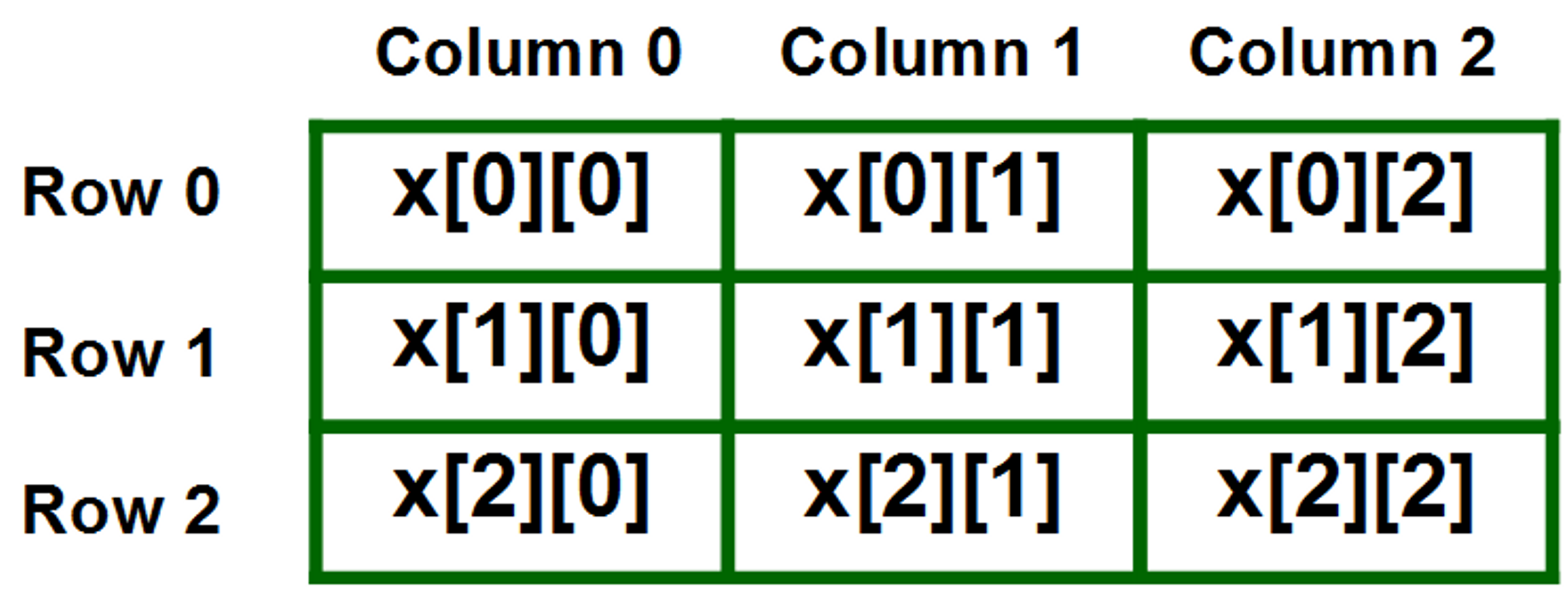
Arrays can also be multidimensional - instead of accessing an element of a one-dimensional list, elements are accessed by two or more indices, as from a matrix. In simpler terms, a matrix is an array of arrays.
To better visualize a multidimensional array , think of an array that has a size of 12, in our case this will be a calendar, one index for every month of the year. Each index will contain another array that will hold all the days in a month. Let’s say we wanted to access the month of May and get the 21st day of the month we would subscript our matrix like so, calendar[4][20]. Matrices are just arrays with arrays inside them so they still follow the 0 index rule which is why even though May is the fifth month of the year we subscript 4 to retrieve it, similarly we subscript 20 to get the 21st day in a month.
Below is an image depicting a multidimensional array, notice the coordinates pattern, this is how these arrays can be accessed. The first subscript deals with column indexes and the second subscript does row indexes.
Three Sum
Final Solution:
def three_sum(array):

  array.sort()

  for i in range(len(array)):

    a = array[i]

    sum = -a
    start = i + 1
    end = len(array)-1

    while(start<end):
      tempSum = array[start] + array[end]

      if(tempSum == sum):
        print("Found 3 elements whose sum is = 0")
        print('Elements are %s, %s and %s.'%(a, array[start], array[end]))
        return
      elif(tempSum<sum):
        start+=1
      else:
        end-=1
Rotate Matrix
Final Solution:
def rotateMatrix(matrix, N):


  for i in range(0, N // 2):

    j = i

    for j in range(j, N - i - 1):

      temp = matrix[i][j]


      matrix[i][j] = matrix[N - 1 - j][i]
      matrix[N - 1 - j][i] = matrix[N - 1 - i][N - 1 - j]
      matrix[N - 1 - i][N - 1 - j] = matrix[j][N - 1 - i]
      matrix[j][N - 1 - i] = temp


  return matrix
Zero Matrix
Final Solution:
def setZeroes(self, matrix):

    """

    :type matrix: List[List[int]]

    :rtype: void Do not return anything, modify matrix in-place instead.

    """

    is_col = False
    R = len(matrix)
    C = len(matrix[0])

    for i in range(R):
      # Since first cell for both first row and first column is the same i.e. matrix[0][0]
      # We can use an additional variable for either the first row/column.
      # For this solution we are using an additional variable for the first column
      # and using matrix[0][0] for the first row.
      if matrix[i][0] == 0:
        is_col = True

      for j in range(1, C):
        # If an element is zero, we set the first element of the corresponding row and column to 0
        if matrix[i][j] == 0:
          matrix[0][j] = 0
          matrix[i][0] = 0

    # Iterate over the array once again and using the first row and first column, update the elements.
    for i in range(1, R):
      for j in range(1, C):
        if not matrix[i][0] or not matrix[0][j]:
          matrix[i][j] = 0

    # See if the first row needs to be set to zero as well
    if matrix[0][0] == 0:
      for j in range(C):
        matrix[0][j] = 0

    # See if the first column needs to be set to zero as well
    if is_col:
      for i in range(R):
        matrix[i][0] = 0
Recursion
Overview
Recursion , simply put, is a function that calls another function.
Think of recursion as a Russian nesting doll, every time you open a doll you’ll find a smaller one inside, this repeats until there are no more dolls.
In order for a recursive function to come to a stop it needs to have a base case . A base case is just a condition, that if met, will stop the recursion. Without a base case the function will call itself repeatedly until the computer runs out of memory. For the Russian doll example, our base case would be if we find no doll within another doll.
After reaching the base case, the functions start to return, with the first function call being returned last.
The reason for our functions being returned in reverse order (Last in first out) is because recursion puts all function calls on a call stack .
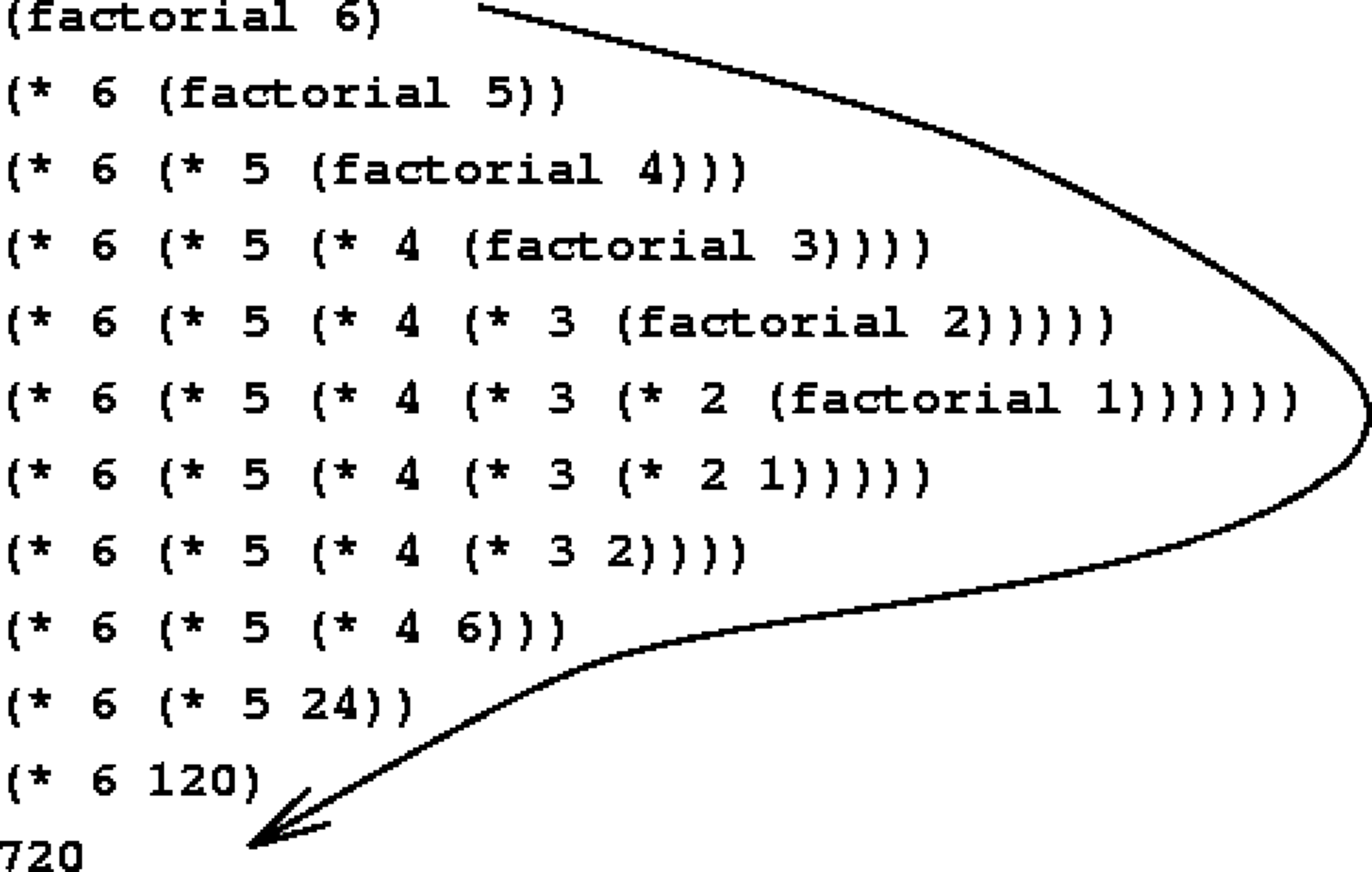
Let’s look at how the call stack works with a real-world example:
If we’re trying to find the sum of 6 factorial then we would need to multiply 6 and all of its subsequent numbers to find our answer. With recursion we can start at 6 and recurse until we hit 1 (our base case), after which we will start performing the math to get our answer (ex: 12345*6). Essentially, recursion does computation on the way back, not while it’s recursing.
Here is an image depicting how our functions will look on our call stack, notice the pattern.
This is pretty much recursion in a nutshell.
Structure of Recursive Implementations
A recursive implementation always has two parts:
-
base case , which is the simplest, smallest instance of the problem, that can’t be decomposed any further. Base cases often correspond to emptiness – the empty string, the empty list, the empty set, the empty tree, zero, etc.
-
recursive step , which decomposes a larger instance of the problem into one or more simpler or smaller instances that can be solved by recursive calls, and then recombines the results of those subproblems to produce the solution to the original problem.
It’s important for the recursive step to transform the problem instance into something smaller, otherwise the recursion may never end. If every recursive step shrinks the problem, and the base case lies at the bottom, then the recursion is guaranteed to be finite.
A recursive implementation may have more than one base case, or more than one recursive step. For example, the Fibonacci function has two base cases, n=0 and n=1.
Recursive Patterns
Identifying certain patterns may help you when deciding if recursion is right for your problem. Recursion is not a one-size-fits-all solution and functions better when it meets certain criteria
Here are 4 patterns to look out for when deciding on a recursive implementation:
Iteration - Recursion can be implemented in any code that uses iteration, like iterating over an array or solving a factorial. Code here can be much more concise.
Subproblems - When doing a problem, if you see subproblems, then that might be a good indicator for a recursive implementation. Examples of subproblems could be counting down from a given number and performing calculations on said numbers. The easiest way to identify subproblems is to see if every recursive call tackles a smaller instance for the same problem, that is a subproblem.
Divide and conquer - “Divide-and-conquer” is most often used to traverse or search data structures such as binary search trees, graphs, and heaps. It also works for many sorting algorithms, like quick sort and heap sort.
DFS - Depth first search is common with trees and graphs, it is used when you need to explore all possible paths in a data structure.
Recursive Use Cases
Some examples use cases for recursion:
- Traversing recursive data structures like trees and graphs.
- Finding files in directory.
- Sorting algorithms, like merge sort
Common Mistakes in Recursive Implementations
Here are two common ways that a recursive implementation can go wrong:
- The base case is missing entirely, or the problem needs more than one base case but not all the base cases are covered.
- The recursive step doesn’t reduce to a smaller subproblem, so the recursion doesn’t converge.
Look for these when you’re debugging.
Memoization
Overview
Memoization is a technique used for speeding up expensive function calls, this is accomplished by ensuring inputs aren’t called more than once by caching previous results.
Let’s take a closer look by running through a simple example:
Below we have a simple (inefficient) function that calculates the nth fibonacci number.
def fib(n):
if (n == 0 || n == 1) return n
return fib(n - 1) + fib(n - 2)
This function has a big problem, it runs in exponential time ( O(2^n) ). The run time is abysmal, even for small inputs. For example, let’s try to find the 50th Fibonacci number, if we did the math, which would be 2^50, this returns 1,125,899,906,842,624. Imagine the amount of calls (and time) needed for a relatively small input.
The problem with the function lies in the recursion:
return fib(n - 1) + fib(n - 2)
What happens here is for every nth number we create two more branches, let’s visualize this by referring to the image below.
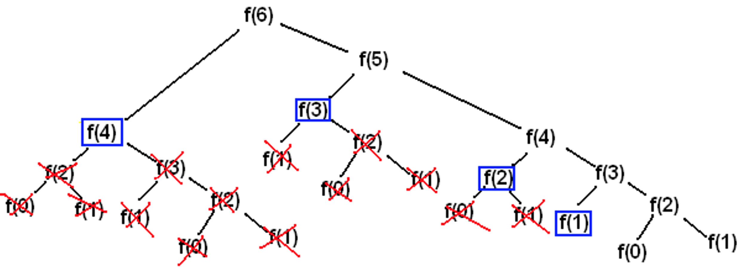
As you can see, some work is being repeated several times. The goal of Memoization is to eliminate all the repeated work by maintaining a cache for previous results.
Whenever we deal with an input, we will first consult the cache, if there is a value we can use, we take it, otherwise we save the current input and continue with our calculations.
Memoization is beneficial when there are common subproblems that are being solved repeatedly. Thus we are able to use some extra storage to save on repeated computation.
Overlapping Subproblems
The image above is also a prime example of overlapping subproblems.
A problem can be said to have overlapping subproblems if you must solve all of its subproblems in a similar manner, rather than generating new problems. Essentially, you are just solving the same problem over and over again.
Given the amount of repeat work our initial approach did, it is safe to say we have a case of overlapping subproblems.
When you have overlapping subproblems then you know you can improve the solution by introducing a strategy like Memoization , or bottoms-up .
Bottoms-Up Approach
Overview
Another strategy for Dynamic Programming problems is known as going bottoms-up, which works well for avoiding recursion. The benefit of this approach would be reducing memory cost on the call stack.
Essentially, going bottoms-up means we start from the beginning by solving small subproblems, we continually do this, using previous subproblems to help solve current subproblems until we’ve reached our final solution.
Recursion operates in an opposite manner, which recurses until the end and builds up the solution backwards.
Imagine you were trying to find the nth fibonacci number, this algorithm is usually done with recursion, but we want to avoid that since it builds up memory on our call stack, which can leaves us prone to a stack overflow. The recursive approach also runs in O(2^n) .
def fib(n):
if (n == 0 || n == 1) return n
return fib(n - 1) + fib(n - 2)
To avoid recursion we can apply the bottoms up strategy to this problem. Instead of relying on our call stack to build our problem or turning to extra space we can just maintain two variables.
In the solution below, we use two variables that hold the two previous fibonacci numbers. Using the variables we can easily make our calculations, update and repeat.
def fibonacci(n):
a  **=**  0

b  **=**  1
if n < 0:
print("Incorrect input")
elif n == 0:
return a
elif n == 1:
return b
else :
for i in range(2,n + 1):
        c  **=**  a  **+**  b

        a  **=**  b

        b  **=**  c
return b
Overall, a much more efficient solution running in O(n) and O(1) space.
Find the Nth Fibonacci Number
Recursive Solution:
def Fibonacci(n):

    if n<=1:
        return n

    else:
        return Fibonacci(n-1)+Fibonacci(n-2)
Memoized Solution:
def fib(n, lookup):

    # Base case
    if n == 0 or n == 1 :
        lookup[n] = n


    # If the value is not calculated previously then calculate it
    if lookup[n] is None:
        lookup[n] = fib(n-1 , lookup) + fib(n-2 , lookup)


    # return the value corresponding to that value of n
    return lookup[n]
Final Solution:
def fibonacci(n):

    a = 0
    b = 1

    if n < 0:
        print("Incorrect input")

    elif n in [0, 1]:
        return n

    else:
        for i in range(2,n+1):
            c = a + b
            a = b
            b = c

        return b
Longest Increasing Subsequence
Final Solution:
def lis(arr):
    n = len(arr)

    # Declare the list (array) for LIS and initialize LIS
    # values for all indexes
    lis = [1]*n

    # Compute optimized LIS values in bottom up manner
    for i in range (1, n):
        for j in range(0, i):
            if arr[i] > arr[j] and lis[i]< lis[j] + 1 :
                lis[i] = lis[j]+1

    # Initialize maximum to 0 to get the maximum of all
    # LIS
    maximum = 0

    # Pick maximum of all LIS values
    for i in range(n):
        maximum = max(maximum, lis[i])

    return maximum
Greedy Algorithms
Overview
Greedy algorithms derive their name from the fact that they choose the most optimal choice at every step in order to find the most optimal answer for a problem. This strategy is effective for some problems like, Huffman coding or the famous Dijkstra’s algorithm, but should not be a go-to strategy for the average algorithm.
Here are a couple properties to consider when deciding if a greedy approach would be desirable for your problem:
- Has Optimal Substructure , in other words, if an optimal solution can be derived from the optimal solution to all of its sub-problems.
- If a problem allows Greedy Choices to be made that will lead to the problems overall optimal solution.
If your problem meets both of these criteria then you may want to look further into adopting a greedy strategy.
Be careful, however, as a greedy approach fails to take in to account the entirety of the problem, only focusing on the immediate information it has at any one step. The issue with this is even if an optimal solution is selected for a sub-problem, there may be more optimal future solutions the greedy approach will invariably overlook.
If you’re finding a greedy approach isn’t working for your problem, you may want to look further into dynamic programming.
Buy & Sell Stocks
Final Solution:
def maxProfit(prices):
  if len(prices) <= 1:
      return 0
  profit = 0
  low = prices[0]
  for i in range(1,len(prices)):
      if prices[i] < low:
          low = prices[i]
      else:
          profit = max(prices[i]-low, profit)
  return profit
Highest Product Of 3
Final Solution:
def maximumProduct(nums):

    min1, min2 = 0, 0

    max1, max2, max3 = 0, 0, 0


    for number in nums:

        if number <= min1:

            min2 = min1

            min1 = number

        elif number <= min2:

            min2 = number

        if number >= max1:

            max3 = max2

            max2 = max1

            max1 = number

        elif number >= max2:

            max3 = max2

            max2 = number

        elif number >= max3:

            max3 = number

    return max(min1 * min2 * max1, max1 * max2 * max3)
Hash Table
Overview
A hash table is a data structure that associates keys with values . The primary operation it supports efficiently is a lookup : given a key (e.g. a person’s name), find the corresponding value (e.g. that person’s telephone number). It works by transforming the key using a hash function into a hash , a number that the hash table uses to locate the desired value. This hash maps directly to a bucket in the array of key/value pairs. The hashing method lets us directly access the storage location for any key/value pair in constant time, on average. Sometimes the hashing method can cause a collision, in this case, if handled correctly, the lookup increases to linear time.
Side note: Hash tables can go by other names such as Map, Hash Map, Dictionary and Hash.
Strengths & Weaknesses
Strengths -
- Key Flexibility - As long as a type is hashable, you can use it as a key.
- Quick Lookup Time - Can retrieve values, on average, in O(1) time.
Weaknesses -
- Unordered - Hash tables don’t order the keys in any particular order, if you’re looking for the smallest key you need to check the entire hash.
- Worst Case Lookup Time - In the event of a collision, our lookup time increases to O(n) time.
Average Case -
Space: O(n)
Insert: O(1)
Lookup: O(1)
Delete: O(1)
Worst Case -
Space: O(n)
Insert: O(n)
Lookup: O(n)
Delete: O(n)
How Do Hash Tables Work
Hash tables and arrays share similar properties, they provide fast lookup to a particular index, or key, in the case of a hash table. Both data structures are known for quick lookup times, in the case of an array as long as you know the index you can find the value at said index very quickly.
You can think of hash tables being built on top of an array, utilizing array indexes to store bits of data. To calculate which index the key will go into hash tables we use hashing functions.
Hashing Functions
Hashing functions are what hash tables use under-the-hood to segment their data. Usually a hash function will take an input and then generate a value, like a number or string. These generated values will function as the key for the values in our hash table.
The key identifies a “bucket” for us to store data, we can access any data by referencing the key.
Sometimes hashing functions can generate the same key twice, which can result in a hash collision.
Hashing functions can get really complex but here is a simple example:
Let’s say you want to store the name of a person and their phone number, the persons name will be the key and the number, the value.
If we want to store a phone number for “Matt” then we can add all the ASCII character codes for each letter and then use an operator known as the modulus (%) to calculate where to store our data.
For example:
M -> 109
A -> 97
T -> 116
T -> 116
109 + 97 + 116 + 116 = 438
Now let’s say the we only have 100 slots in our array, we can use the size of our array to mod our sum to find out which index to store our data.
438 % 100 = 38
Given this result, we will store our data in index 38.
An important note, the array is just an analogy to help understand how a hash table stores its data. Most hash tables don’t have a fixed size but hashing functions are very unique, and intuitive and can take many forms, the primary goal being to properly distribute data and avoid collisions.
Hash Table Collisions
A good hashing function is paramount to avoiding hash collisions. Collisions occur when the hashing function generates the same “index” for a piece of data, and then you end up with multiple pieces of data in the same index.
Most programming languages have built-in hash tables that can handle collisions in a number of ways, some examples are, generating a linked list at the index to accommodate new data in a linear matter, or even using a tree structure to allow really quick lookup times when looking in an index with collisions.
When a collision happens our hash table operates in the worst case, increasing lookup times for indexes with multiple values.

Sets
Like a hash table, in the sense that it is an unordered data structure, a set only holds unique values. Unlike the hash table, instead of retrieving an item by referencing a key, sets are typically used for checking membership.
For example, if you were to add multiple strings to a set and then check if a certain value exists, then that would be considered checking for membership.
car_brands = set()
car_brands.add(“Tesla”)
car_brands.add(“Lamborghini”)
car_brands.add(“Volkswagen”)
‘Tesla’ in car_brands # True
‘Jeep’ in car_brands # False
Palindrome Permutation
Final Solution:
def hasPalindromePermutation(theString):
    unpairedCharacters = set()


    for char in list(theString):
      if char in unpairedCharacters:
        unpairedCharacters.remove(char)
      else:
        unpairedCharacters.add(char)


    return len(unpairedCharacters) <= 1
Longest Consecutive Sequence
Final Solution:
def longestConsecutive(nums):

    longest_streak = 0

    num_set = set(nums)


    for num in num_set:

      if num - 1 not in num_set:

        current_num = num

        current_streak = 1


        while current_num + 1 in num_set:

          current_num += 1

          current_streak += 1


        longest_streak = max(longest_streak, current_streak)


    return longest_streak
Linked List
Overview
A linked list is a linear data structure made up of a series of objects, each object points to the next and so on.
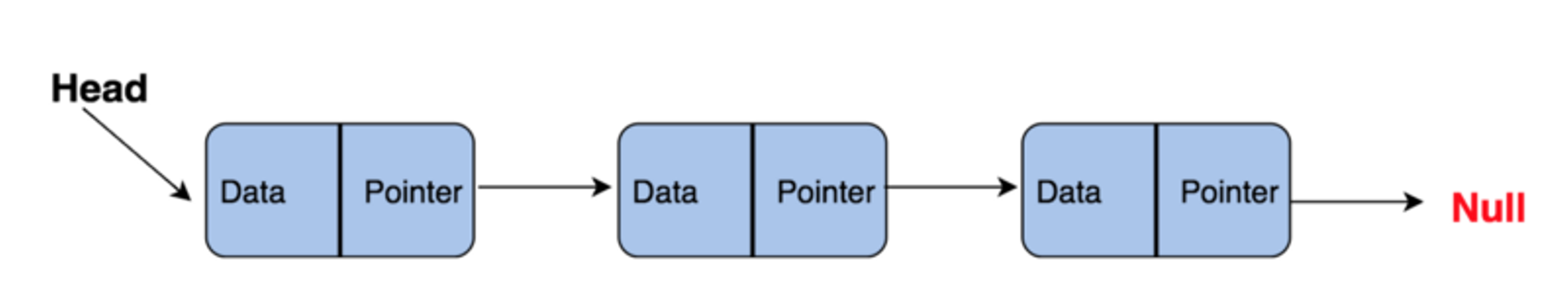
An element in a linked list is called a node , the first node, the head and the final node, the tail .
Strengths & Weaknesses
Strengths -
- Inserting and Deleting - Data does not require us to move/shift subsequent data elements.
- Fast Appending and Prepending - Adding elements to either end is a O(1) operation.
- Flexibility - Can add or remove as many elements as you wish, no need to declare ahead of time.
Weaknesses -
- Linear Lookup Time - Looking for a particular element is an O(n) operation as you must traverse the list from beginning to end, or until element is found.
Worst Case -
Space: O(n)
Lookup: O(n)
Prepend: O(1)
Append: O(1)
Insert: O(n)
Delete: O(n)
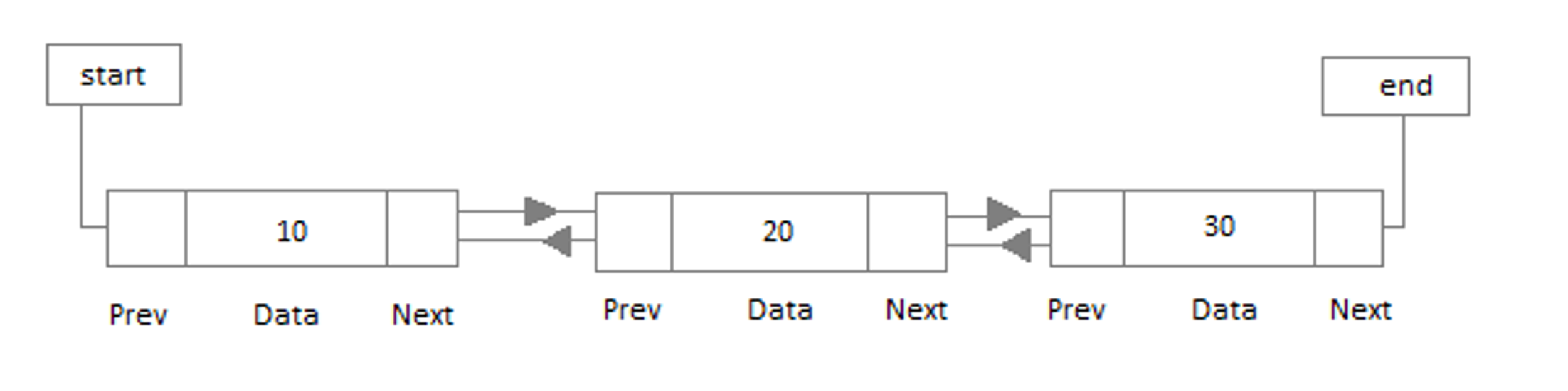
Doubly Linked Lists
Similar to a linked list, a doubly linked list has pointers to the node next to it and previous to it . The benefit of a doubly linked list is we can now traverse the list both forwards and backwards. This can be helpful if we ever need to quickly go back from a current node to check previous data.
Reverse A Linked List
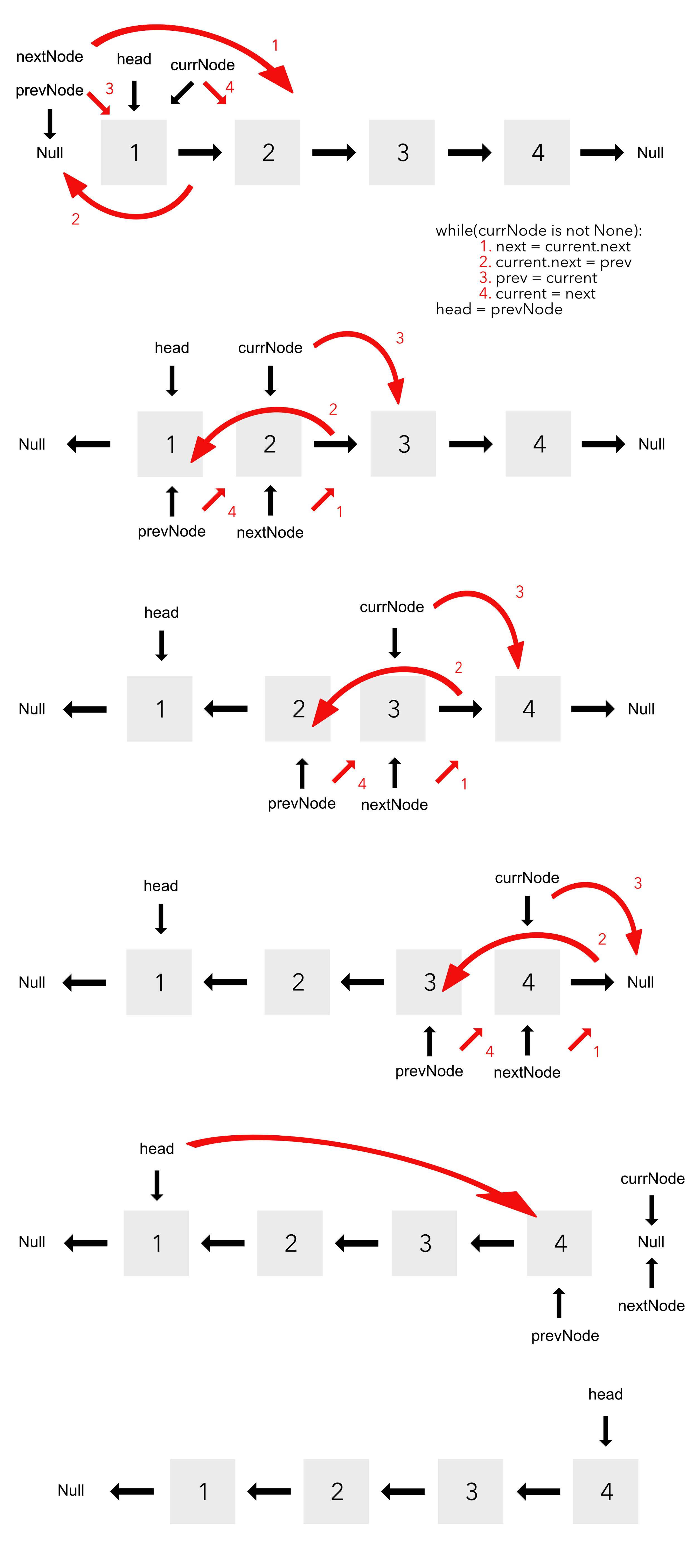
Final Solution:
def reverse(head):

    prev = None

    current = head

    while(current is not None):

        next = current.next

        current.next = prev

        prev = current

        current = next

    self.head = prev

  return prev
Determine If Linked List Is A Palindrome
Final Solution:
def isListPalindrome(self):
	""" Check if linked list is palindrome and return True/False."""
	node = self.head
	fast = node
	prev = None


	# prev approaches to middle of list till fast reaches end or None
	while fast and fast.next:
	    fast = fast.next.next
	    temp = node.next   #reverse elemets of first half of list
	    node.next = prev
	    prev = node
	    node = temp


	if fast:  # in case of odd num elements
	    tail = node.next
	else:    # in case of even num elements
	    tail = node


	while prev:
	    # compare reverse element and next half elements
	    if prev.val == tail.val:
	        tail = tail.next
	        prev = prev.next
	    else:
	        return False
	return True
Add Two Numbers Represented As Linked Lists
Final Solution:
# Definition for singly-linked list.
class ListNode(object):
	def __init__(self, x):
	    self.val = x
	    self.next = None

class Solution(object):
	def addTwoNumbers(self, l1, l2):
	    """
	    :type l1: ListNode
	    :type l2: ListNode
	    :rtype: ListNode
	    """
	    result = ListNode(0)
	    result_tail = result
	    carry = 0

	    while l1 or l2 or carry:
	        val1  = (l1.val if l1 else 0)
	        val2  = (l2.val if l2 else 0)
	        carry, out = divmod(val1+val2 + carry, 10)

	        result_tail.next = ListNode(out)
	        result_tail = result_tail.next

	        l1 = (l1.next if l1 else None)
	        l2 = (l2.next if l2 else None)

	    return result.next
Reverse K Groups In Linked List
Final Solution:
# Reverses the linked list in groups of size k
# and returns the pointer to the new head node.
def reverse(self, k = 1):
    if self.head is None:
        return


    curr = self.head
    prev = None
    new_stack = []
    while curr is not None:
        val = 0

        # Terminate the loop whichever comes first
        # either current == None or value >= k
        while curr is not None and val < k:
            new_stack.append(curr.data)
            curr = curr.next
            val += 1


        # Now pop the elements of stack one by one
        while new_stack:

            # If final list has not been started yet.
            if prev is None:
                prev = Node(new_stack.pop())
                self.head = prev
            else:
                prev.next = Node(new_stack.pop())
                prev = prev.next

    # Next of last element will point to None.
    prev.next = None
    return self.head
Stack
Overview
A stack is a basic data structure that can be logically thought of as a linear structure represented by a real physical stack or pile, a structure where insertion and deletion of items takes place at only one end, at the top of the stack.
The implementation of a stack follows the LIFO principle (Last In First Out) to demonstrate the way it accesses data, the basic concept can be illustrated by thinking of your data set as a stack of plates or books where you can only take the top item off the stack in order to remove things from it.
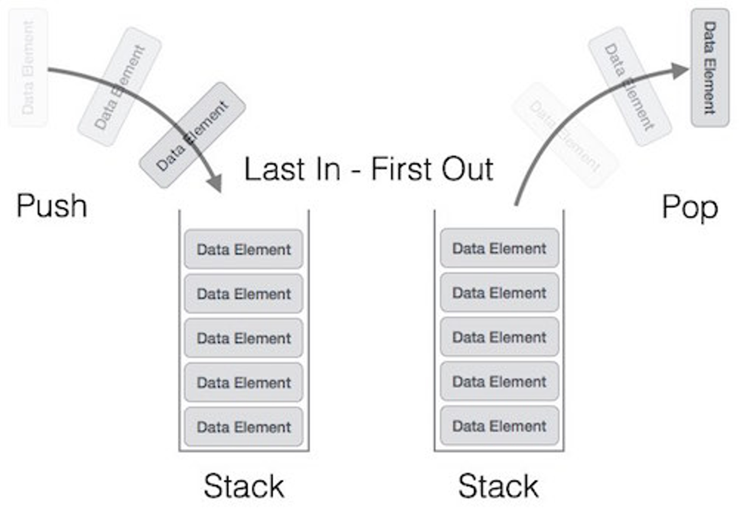
There are basically three operations that can be performed on stacks.
- Push - Inserting items into the stack.
- Pop - Deleting items from the stack.
- Peek - Displaying the top-most item in stack at any given time.
A stack can usually be implemented by a dynamic array or a linked list, both are good choices.
A good use case for a stack would be when performing Depth First Searches (DFS), usually on Trees or Graphs.
Strengths & Weaknesses
Strengths -
- Fast Operations - Pushing or popping items onto the stack takes O(1) time.
- Not Easily Corrupted - Items can’t be inserted in the middle of the stack, thus protecting it from corruption.
- Enforces Order - Depending on your use case, the LIFO principle can be beneficial as the data is handled in a specific way, unlike other data structures, such as arrays.
Weaknesses -
- Random Access Is Impossible - Items can only be pushed or popped off, you can’t access the bottom of the stack (or any other item) by imply querying it, must go through each item one by one. Might not suit certain use cases.
- Stack Overflow - Adding too many objects to a stack opens the risk of a stack overflow happening. Usually as a result of running out of memory.
Worst Case -
Space: O(n)
Push: O(1)
Pop: O(1)
Peek: O(1)
Call Stack
A call stack is a stack used for managing function calls in our programs. The purpose of the call stack is to manage all the subroutines our program is running and when to return control to previous operations when the current operation finishes executing.
Call stack space is usually limited, so if overloaded, could run the risk of a stack overflow.
Queue
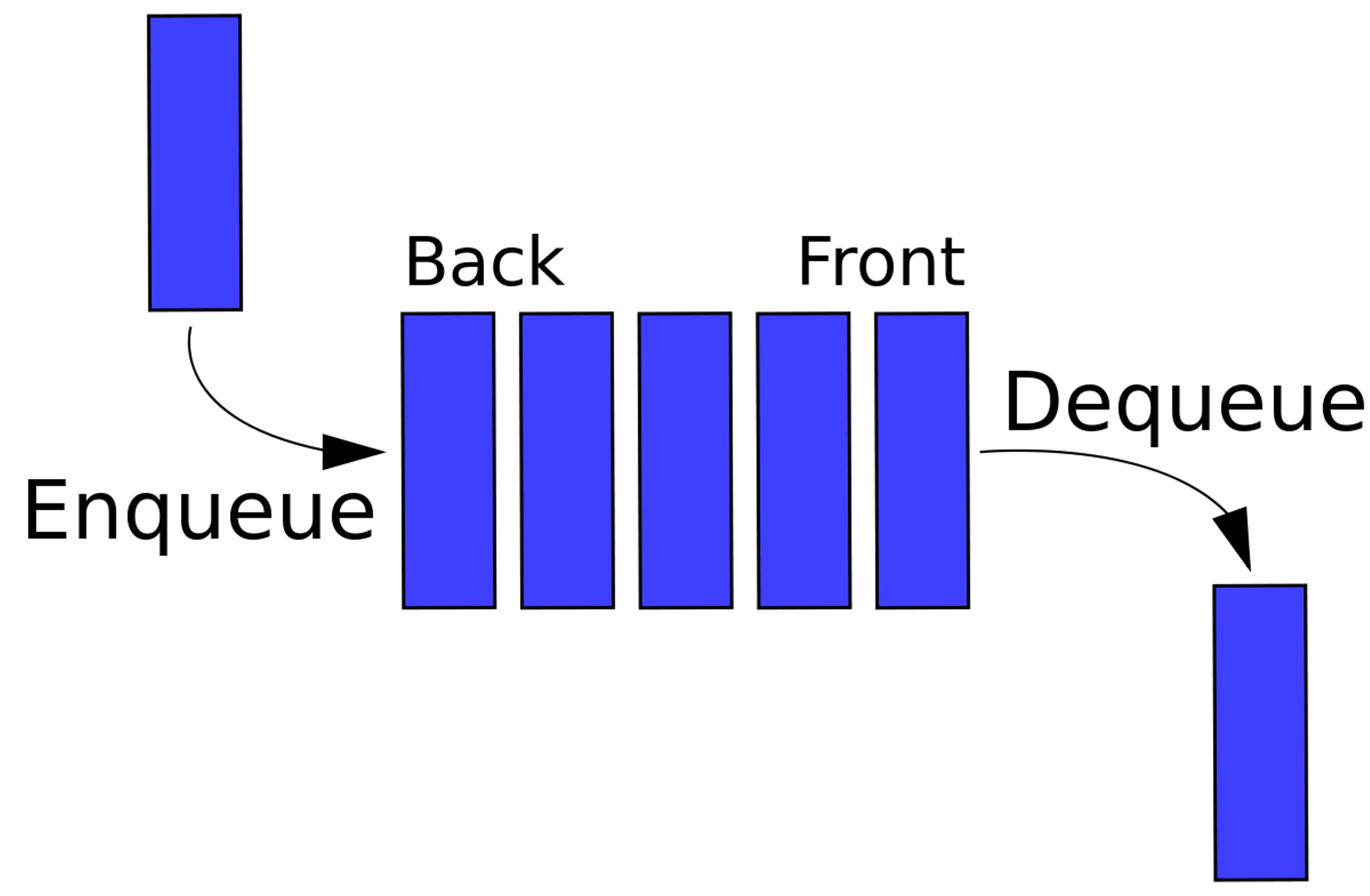
Overview
A queue is a basic data structure that is used throughout programming. You can think of it as a line in a grocery store. The first one in the line is the first one to be served.Just like a queue.
A queue is also called a FIFO (First In First Out) to demonstrate the way it accesses data.
Queues can be best represented with linked lists.
Some good real-world use cases for queues are when preforming Breadth First Searches (BFS), or when scheduling several processes to run on your computer. The queue has many applications.
Worst Case -
Space: O(n)
Enqueue: O(1)
Dequeue: O(1)
Peek: O(1)
Strengths & Weaknesses
Strengths -
- Fast Operations - All operations takes O(1) time.
- Not Easily Corrupted - Items can’t be inserted in the middle of the stack, thus protecting it from corruption.
- Enforces Order - Depending on your use case, the FIFO principle can be beneficial as the data is handled in a specific way, unlike other data structures, such as arrays.
Weaknesses -
- Random Access Is Impossible - Items can only be enqueued or dequeued, you can’t access the middle of the queue without removing some items first.
Implement A Queue w/ Two Stacks
Final Solution:
class MyQueue(object):

    def __init__(self):
        self.stack1 = []
        self.stack2 = []

    def enqueue(self, item):
        self.stack1.append(item)

    def dequeue(self):
        if len(self.stack2) == 0:

            # Move items from in_stack to out_stack, reversing order
            while len(self.stack1) > 0:
                newItem = self.stack1.pop()
                self.stack2.append(newItem)

            # If out_stack is still empty, raise an error
            if len(self.stack2) == 0:
                raise IndexError("Can't dequeue from empty queue!")

        return self.stack2.pop()
Get Minimum Element From Stack
Final Solution:
class MinStack(object):

    def __init__(self):
        self.stack = Stack()
        self.min_stack = Stack()


    def push(self, item):
        """Add a new item onto the top of our stack."""
        self.stack.push(item)


        # If the item is greater than or equal to the last item in maxes_stack,
        # it's the new max! So we'll add it to maxes_stack.
        if self.min_stack.peek() is None or item <= self.min_stack.peek():
            self.min_stack.push(item)

    def pop(self):
        """Remove and return the top item from our stack."""
        item = self.stack.pop()

        # If it equals the top item in maxes_stack, they must have been pushed
        # in together. So we'll pop it out of maxes_stack too.
        if item == self.min_stack.peek():
            self.min_stack.pop()

        return item

    def getMin(self):
        """The last item in maxes_stack is the max item in our stack."""
        return self.min_stack.peek()
Balanced Brackets
Final Solution:
PAIRINGS = {

  '(': ')',

  '{': '}',

  '[': ']'

}


def is_balanced(symbols):

  stack = []

  for s in symbols:

    if s in PAIRINGS.keys():

      stack.append(s)

      continue

    try:

      expected_opening_symbol = stack.pop()

    except IndexError: # too many closing symbols

      return False

    if s != PAIRINGS[expected_opening_symbol]: # mismatch

      return False

  return len(stack) == 0