Tree
Overview
A tree is a data structure comprised of nodes, with an element of the tree designated as the root. Trees are generally defined as recursive data structures because each node consists of a value and then has connections to “child” nodes, who in turn also act as roots to their own child nodes and so on.
Tree nodes have many useful properties. The depth of a node is the length of the path (or the number of edges) from the root to that node. The height of a node is the longest path from that node to its leaves. The height of a tree is the height of the root. A leaf node has no children—its only path is up to its parent.

The image above depicts a “perfect” tree, or in other words, where every node has two child nodes. This tree is completely full. The image also shows how the number of nodes at every level of the tree doubles from the previous.
At any given time, our “perfect” tree contains half of the total sum of nodes on the last level of the tree.
We can calculate the number of nodes in our tree by simply counting all the nodes in the last level, multiplying by 2 and then subtracting 1.
n = 2^h-1
This example should highlight the relationship between a “perfect” binary tree’s height and the number of nodes it contains.
Types Of Trees
Binary Tree - Each node can have zero, one or two child nodes. The binary tree makes operations simple and efficient.
Binary Search Tree - A binary tree where any left child node has a value less than its parent node and any right child node has a value greater than or equal to that of its parent node.
Tree Traversal Mechanisms
When dealing with binary trees, you have a few options for visiting nodes: preorder , postorder and in-order . All traversal methods accomplish the same goal, the difference is in how they traverse the current node and its children.
preorder : Current node, left subtree, right subtree
postorder : Left subtree, right subtree, current node
in-order : Left subtree, current node, right subtree
Here are examples of the different tree traversal mechanisms on a binary search tree:
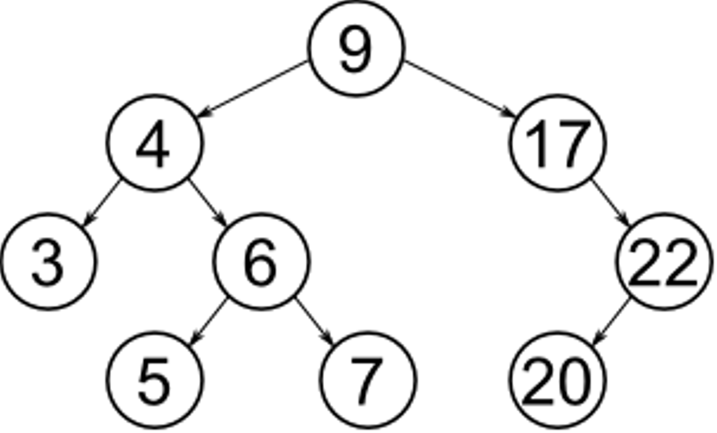
preorder : 9, 4, 3, 6, 5, 7, 17, 22, 20
postorder : 3, 5, 7, 6, 4, 20, 22, 17, 9
in-order : 3, 4, 5, 6, 7, 9, 17, 20, 22
Average Case -
Space: O(n)
Search: O(log n)
Insert: O(log n)
Delete: O(log n)
Worst Case -
Space: O(n)
Search: O(n)
Insert: O(n)
Delete: O(n)
Why Use Trees?
Trees are diverse data structures with many applications in the real world, here are a few:
- You may want to store information in a hierarchical manner, a simple example would be a file system on your computer (You would have a home directory then sub directories etc…).
- If quick insert/deletes are important then a tree might be a viable option, they generally perform these operations faster than an array.
- If data is organized in a binary search tree then lookup times for our data will consistently run in O(log n) .
Graph
Overview
A graph is a data structure that is made of a network of interconnected items.
Each item in the graph is a node (aka vertex ), and is connected to other nodes by edges .
Essentially, a graph is just a set of nodes with relations to other nodes.

Graphs are ubiquitous in computer science. They are used to model real-world systems such as the Internet (each node represents a router and each edge represents a connection between routers); airline connections (each node is an airport and each edge is a flight); or a city road network (each node represents an intersection and each edge represents a block).
The strength of a graph shines when dealing with data that needs to be connected. If you’re ever dealing with data that needs to be linked together in some way, a graph might be a good choice.
As for weaknesses , when traversing graphs some algorithms run in O(n * log(n)). If your graph is large, then running these algorithms may not be the most efficient approach.
Graph Terminology
There are many terms used to classify a graph, it’s important to know the difference so you can apply them to the appropriate use case.
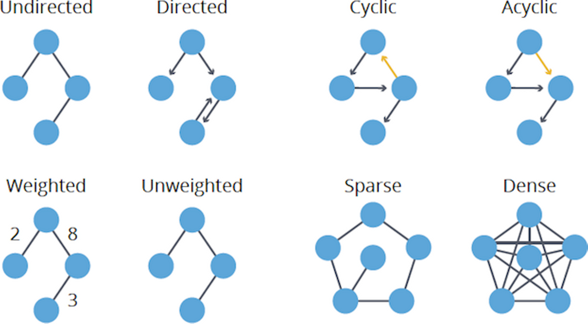
Directed or undirected
These types of graphs are classified by whether their edges have a direction.
-
Directed Graphs : Each edge can only be traversed in one direction.
-
Undirected Graphs: Each edge can be traversed in either direction.
Cyclic or acyclic
These types of graphs are classified by whether they contain a cycle or not.
-
Cyclic Graphs : Contains a cycle.
-
Acyclic Graphs: Does not contain a cycle.
Weighted or unweighted
These types of graphs are classified by whether their edges have weight or not.
-
Weighted Graphs : Edges contain weight, defined by a numerical value. Usually used for showing the cost of traversing the edges between nodes.
-
Unweighted Graphs: Edges contain no weight.
Representations
Edge List
An edge list is an unordered list of all edges in a graph.
Let’s look at an example to understand how an edge list tracks edges:
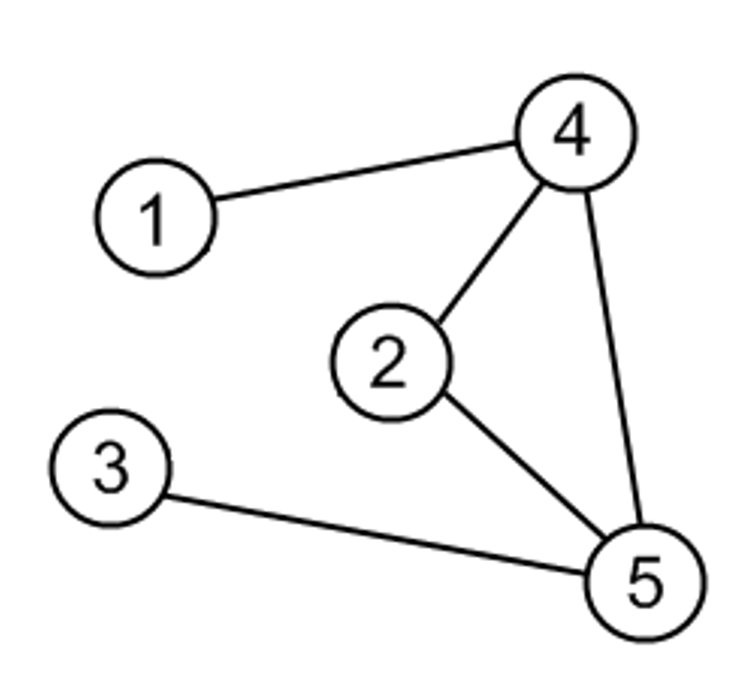
Here is a list that tracks all edges from our example.
edge_list = [ [1, 4], [2, 4], [2, 5], [3, 5], [4, 5] ]
Node 2 has edges to 4 and 5, which is represented by [2, 4] and [2, 5] in the list, respectively.
Advantages -
- Easy to loop over all edges.
Disadvantages -
- Hard to determine how many edges a particular node touches.
- Hard to determine if edge exists between A and B nodes.
Adjacency List
There are many ways to implement an adjacency list. The most common implementation is to maintain a list where each index represents a node and the value at the index contains all of the nodes neighbors.
adjacency_list = [
[],
[4],
[4, 5],
[5],
[5]
]
In the list you can see node 3 only has a connection to node 5. If you retrieve the value from adjacency_list[3] you get 5.
Another implementation uses a dictionary (hash map), the concept is similar:
adjacency_list = {
0: [],
1: [4],
2: [4, 5],
3: [5],
4: [5]
}
One advantage of using a dictionary is the keys can represent other values besides integers, let’s say your nodes use letters, this approach can accommodate that.
Advantages -
- New nodes are added easily.
- Easy to determine the neighbors of a particular node.
Disadvantages -
- Determining if edge exists between two nodes can take O(n) time, n being the size of the list at that index.
Adjacency Matrix
To determine if two nodes are adjacent to each other we must find the coordinates. Since we’re dealing with a matrix we must have ‘x’ and ‘y’ values, which determine the appropriate row and column.
Below we have a matrix of 0’s and 1’s, which represent true or false, respectively.
adjacency_matrix = [
[0, 0, 0, 0, 0, 0],
[0, 0, 0, 0, 1, 0],
[0, 0, 0, 0, 1, 1],
[0, 0, 0, 0, 0, 1],
[0, 1, 1, 0, 0, 1],
[0, 0, 1, 1, 1, 0]
]
If we want to check if node 5 has any adjacent nodes we can see in adjacency_matrix[5] that there are adjacent nodes at indexes 2, 3 and 4 (represented as adjacency_matrix[5][2] , adjacency_matrix[5][3] and adjacency_matrix[5][4] , respectively).
Our image above shows that node 5 is indeed connected to node 2, 3 and 4.
The memory use of an adjacency matrix is O(n^2).
Advantages -
- Quick to determine if an edge exists between two nodes.
Disadvantages -
- Consumes a lot of memory if graph is sparse.
- Matrix can contain a lot of redundant information.
Breadth-First Search (BFS)
Overview
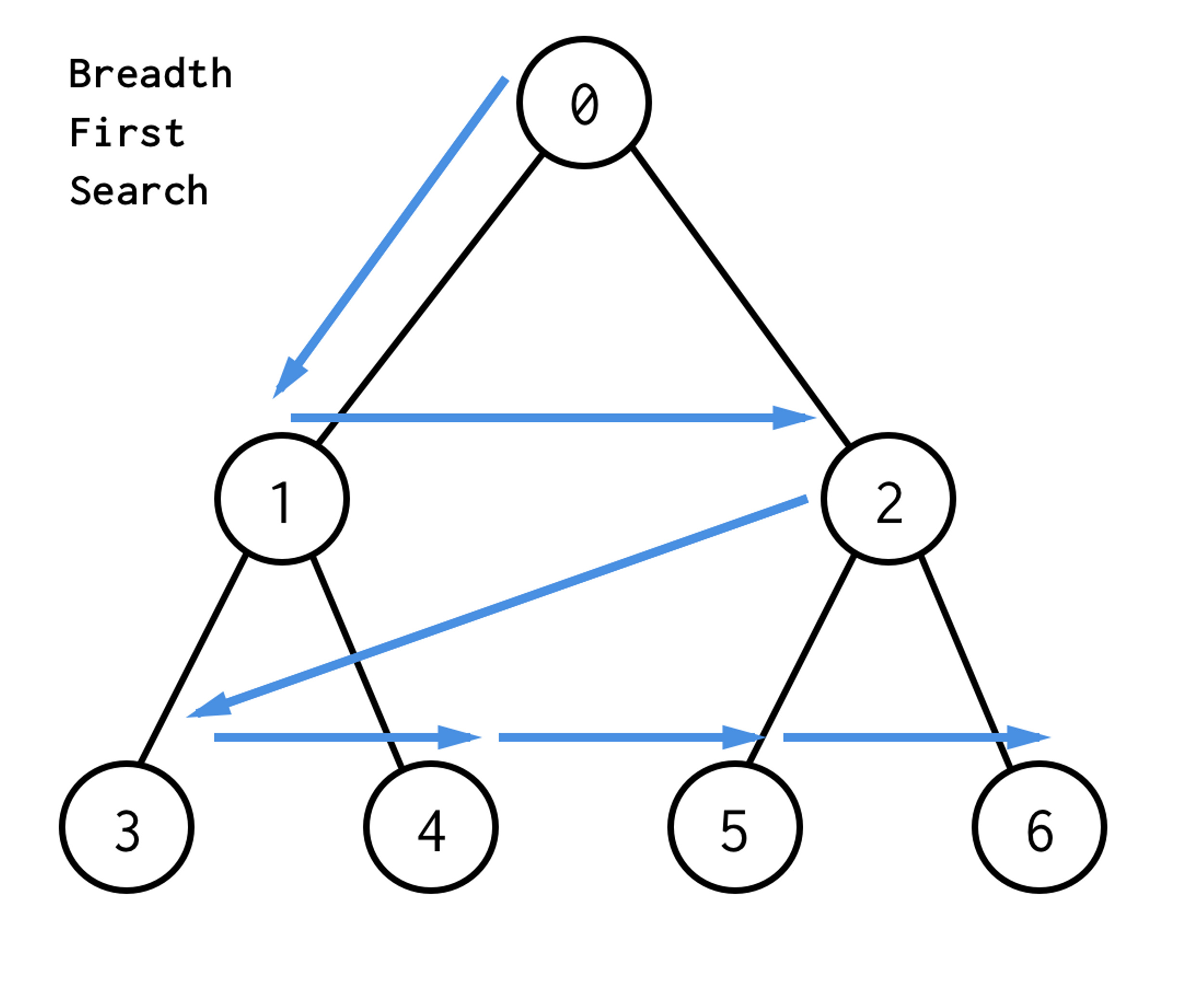
Breadth-first search (BFS) is the most common approach for traversing graphs. After selecting a starter node, using BFS you will begin to traverse the graph (or tree) layer by layer, this means exploring the immediate neighbor nodes before moving on further.
A BFS implementation is accomplished by maintaining a queue where we can enqueue the first layer of nodes and process them before repeating the process with the next layer.
Here is an image depicting how BFS would look on a tree structure:
Advantages of BFS
- Best choice for finding the shortest path between two nodes.
Disadvantages of BFS
- BFS, on average, requires more memory than DFS. This is because all nodes of a current level must be processed before moving on.
- If graph/tree is large, then traversal can be time consuming.
Depth-First Search (DFS)
Overview
Depth-first search (DFS) is another strategy for traversing graphs. Instead of traversing layer by layer, DFS explores a path as much as possible before backing up and exploring another path until the end.
DFS uses the idea of backtracking to ensure every path is explored.
A DFS implementation can be achieved by using a stack. We start at a node and keep pushing adjacent nodes on to the stack until there is no more nodes in a path, we can then pop nodes off and backtrack. While backtracking, if we encounter more unexplored paths then we begin pushing the new nodes on to the stack.
Here is an image depicting how DFS would look on a tree structure:

Advantages of DFS
- DFS can be implemented easily with recursion, which works well with both trees and graphs.
- DFS, on average, requires less memory then BFS to implement.
- DFS is good for exhausting all possible choices in a structure.
Disadvantages of DFS
- DFS is not guaranteed to find the shortest path to a node, unlike BFS.
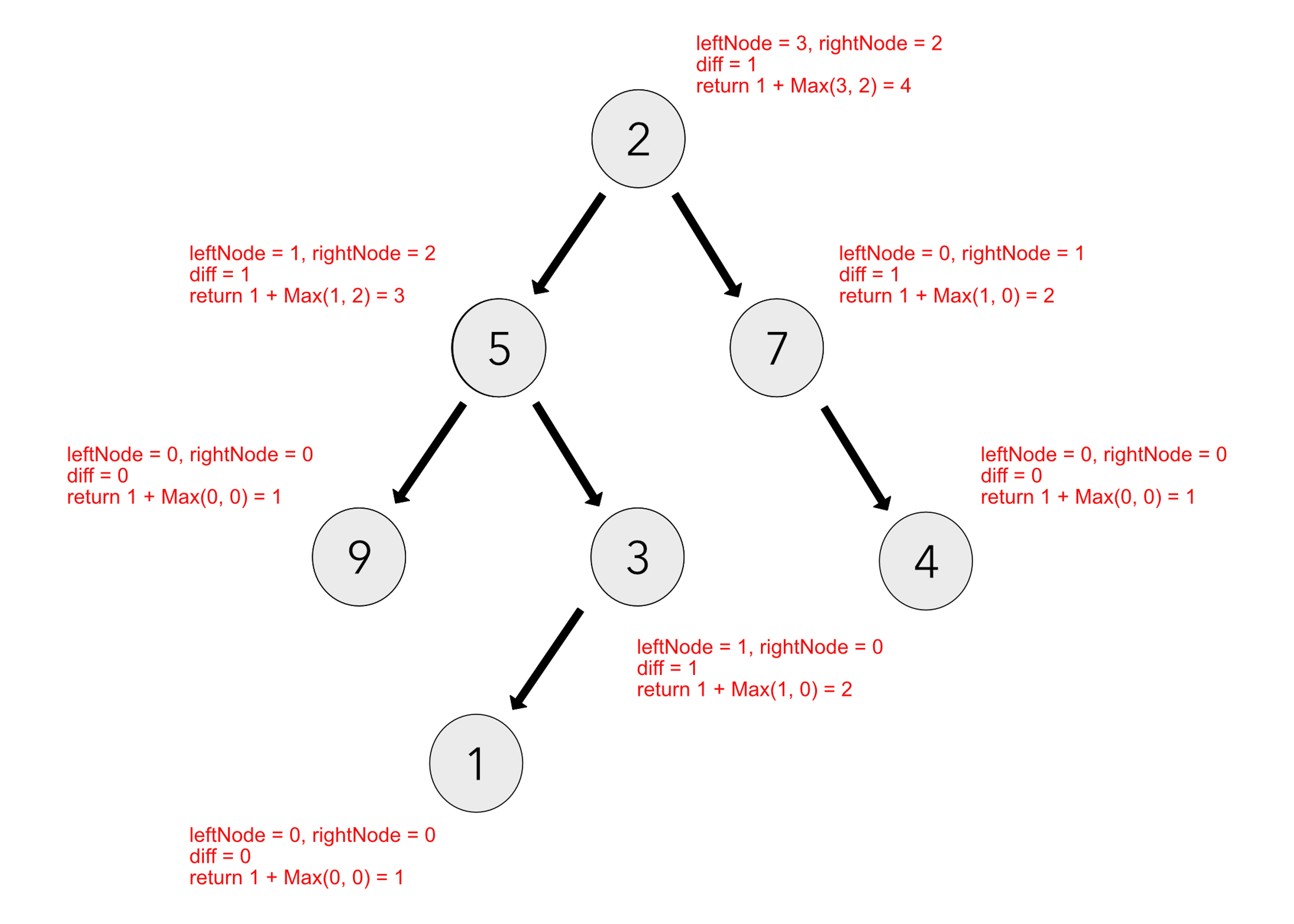
Check If Binary Tree Is Balanced
Final Solution:
def is_balanced(self, root):
    return self.is_balanced_helper(root)[0]


def is_balanced_helper(self, root):
    if root is None:
        return (True, 0)

    left_result, left_height = self.is_balanced_helper(root.left)
    right_result, right_height = self.is_balanced_helper(root.right)


    return (left_result and right_result and abs(left_height - right_height) <= 1, max(left_height, right_height) + 1)
Here is an example of a balanced tree:
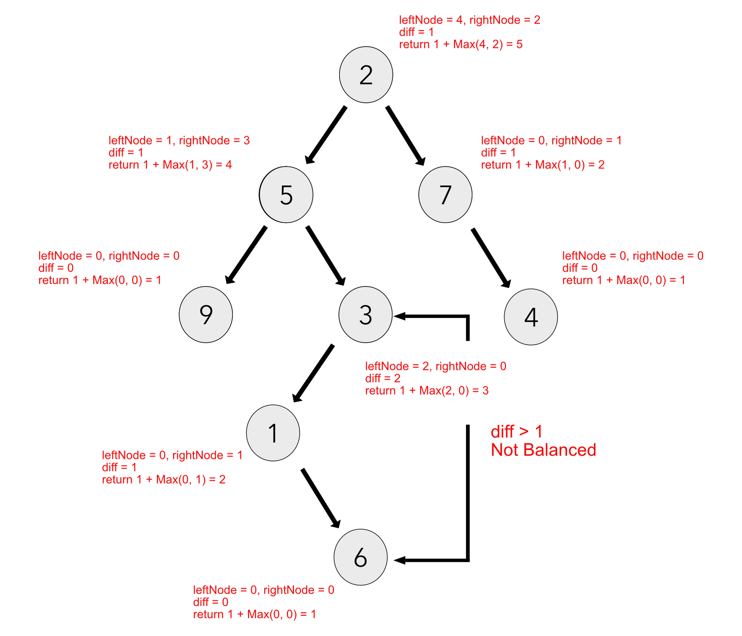
Here is an example of an unbalanced tree:
Find Second Largest Element In BST
Recursive Solution:
def find_largest(root_node):

  if root_node is None:

    raise ValueError('Tree must have at least 1 node')

  if root_node.right is not None:

    return find_largest(root_node.right)

  return root_node.value


def find_second_largest(root_node):

  if (root_node is None or

      (root_node.left is None and root_node.right is None)):

    raise ValueError('Tree must have at least 2 nodes')


  if root_node.left and not root_node.right:

    return find_largest(root_node.left)


  if (root_node.right and

      not root_node.right.left and

      not root_node.right.right):

    return root_node.value


  return find_second_largest(root_node.right)
Iterative Solution:
def find_largest(root_node):

  current = root_node

  while current:

    if not current.right:

      return current.value

    current = current.right


def find_second_largest(root_node):

  if (root_node is None or

      (root_node.left is None and root_node.right is None)):

    raise ValueError('Tree must have at least 2 nodes')


  current = root_node

  while current:

    if current.left and not current.right:

      return find_largest(current.left)


    if (current.right and

        not current.right.left and

        not current.right.right):

      return current.value


    current = current.right
Lowest Common Ancestor
Final Solution:
def findLCA(root, n1, n2):

    # Base Case
    if root is None:
        return None

    # If node matches either of our targets, return root
    if root.data == n1 or root.data == n2:
        return root

    # Look for keys in left and right subtrees
    left_lca = findLCA(root.left, n1, n2)
    right_lca = findLCA(root.right, n1, n2)

    # If both the left and right children return not null values
    # then we know this node is the LCA
    if left_lca and right_lca:
        return root

    # Otherwise check if left subtree or right subtree is LCA
    return left_lca if left_lca is not None else right_lca
Invert Binary Tree
Iterative Solution:
def invertTree(self, root):

    q = deque() # a deque is similar to queue functionality-wise

    q.append(root)

    while q:

        node = q.popleft()

        if node:

            node.left, node.right = node.right, node.left

            q.append(node.left)

            q.append(node.right)

    return root
Recursive Solution:
def invertTree(self, root):

    """

    :type root: TreeNode

    :rtype: TreeNode

    """

    if not root:

      return None


    res = TreeNode(root.val)

    if root.right:

      res.left = self.invertTree(root.right)

    else:

      res.left = None


    if root.left:

      res.right = self.invertTree(root.left)

    else:

      res.right = None


    return res
Key Characteristics Of Distributed Systems
There are several characteristics we can use to develop distributed systems, they include topics, such as, scalability , reliability , availability , efficiency and serviceability . Let’s review them:
Scalability
Scaleability describes a systems ability to keep up with an increased demand or work load by adding more resources. When a service starts to acquire more users, perform more transactions or add more storage capacity there may be a noticeable hit to performance. In order for a system to truly be scaleable it must be built in a way that doesn’t need to be redesigned to maintain effective performance after an increase in workload.
When designing a system for scaleability you will inevitably come to a point when you need to decide whether to scale a service horizontally or vertically. Each method has its merits, though, more often than not, horizontal scaleability is the default choice for many scaling decisions.
Let’s discuss both horizontal and vertical scaling more in-depth:
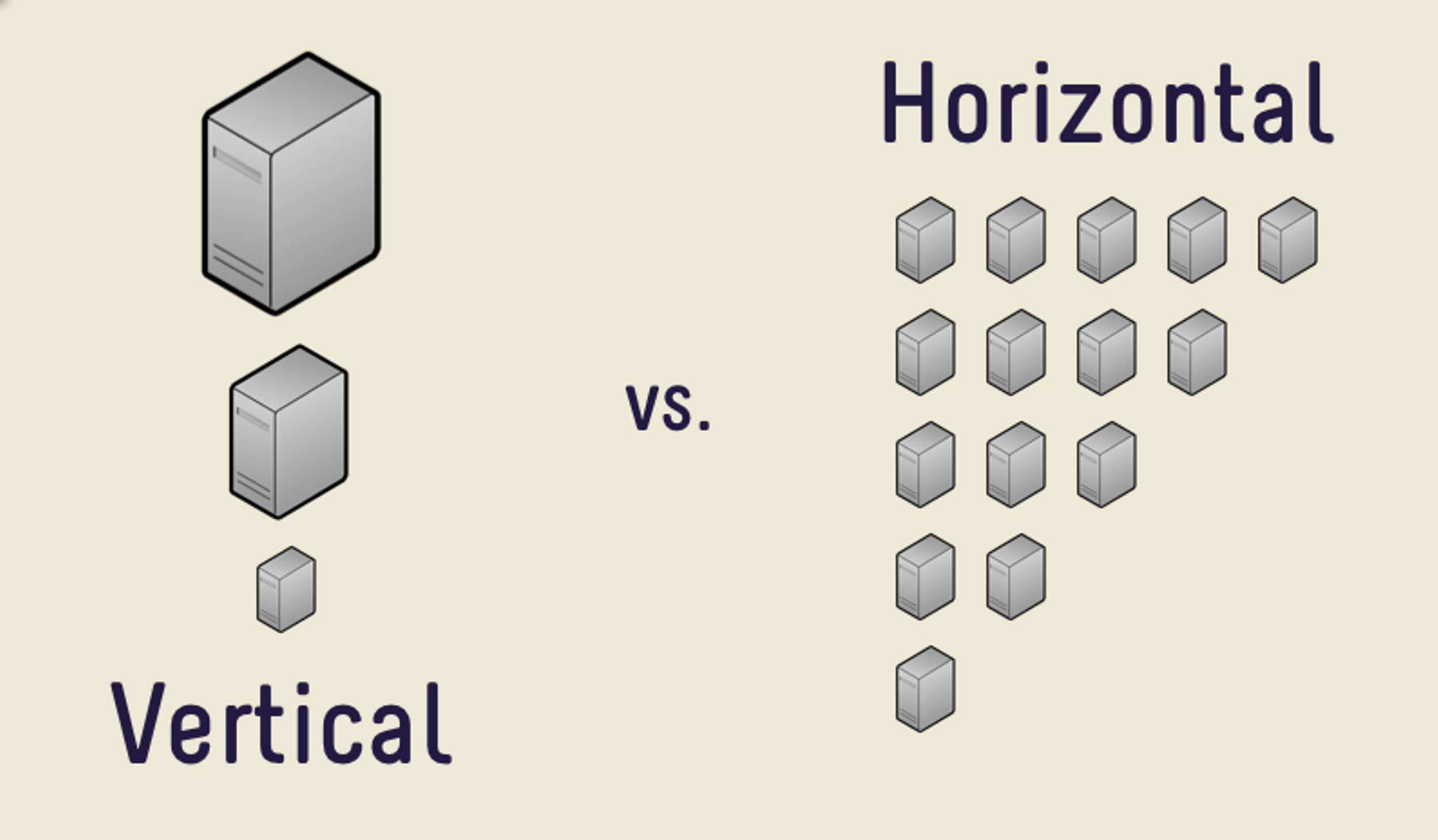
Horizontal Scaling
Horizontal scaling simply means to scale by adding more machines to your pool of resources. Usually this means acquiring more servers to help distribute the increased workload.
One of the benefits to horizontal scaling is that we can dynamically add more servers when we need it.
Some good examples of horizontally scaling technologies are Cassandra, MongoDB, as they both provide an easy way to scale horizontally by adding more machines to meet growing needs.
Vertical Scaling
Vertical scaling means that you scale by adding more power (CPU, RAM, Storage, etc.) to an existing server. Essentially, increasing the capability of a single machine.
There is a downside to vertical scaling which is often limited to the capacity of a single machine, scaling beyond that capacity often involves downtime and comes with an upper limit.
A good example of vertical scaling is MySQL as it allows for an easy way to scale vertically by switching from smaller to bigger machines.
Below is a visual representation of horizontal and vertical scaling:
Reliability
By definition, reliability is the probability a system will fail in a given period. In simple terms, a distributed system is considered reliable if it keeps delivering its services even when one or several of its software or hardware components fail. Reliability represents one of the main characteristics of any distributed system, since in such systems any failing machine can always be replaced by another healthy one, ensuring the completion of the requested task.
Take the example of a large electronic commerce store (like Amazon), where one of the primary requirement is that any user transaction should never be canceled due to a failure of the machine that is running that transaction. For instance, if a user has added an item to their shopping cart, the system is expected not to lose it. A reliable distributed system achieves this through redundancy of both the software components and data. If the server carrying the user’s shopping cart fails, another server that has the exact replica of the shopping cart should replace it.
Obviously, redundancy has a cost and a reliable system has to pay that to achieve such resilience for services by eliminating every single point of failure.
Availability
Availability is the simple measure of the percentage of time that a service, device or resource remains operational under normal conditions. A real-world example of availability would be operating aircrafts, an aircraft that can be flown for many hours a month without much downtime can be said to have a high availability.
Reliability is availability over time considering the full range of possible real-world conditions that can occur. An aircraft that can make it through any type of weather safely is more reliable than one that has vulnerabilities to possible conditions.
Reliability vs. Availability
People sometimes confuse reliability and availability and think they are one and the same, they are in fact distinct. If a system is reliable, then we can also say it is available, however, it is not the same the other way around. In essence, a highly reliable system contributes to a high availability.
In the event we had system that was highly available but had low reliability, the customer might not notice any difference initially. Since our system would not be reliable, if a security breach occurred, it could potentially bring down the entire system, thus ruining any availability the system had.
When building distributed systems it is crucial to make the system both reliable and available.
Efficiency
How do we estimate the efficiency of a distributed system? Assume an operation that runs in a distributed manner, and delivers a set of items as result. Two usual measures of its efficiency are the response time (or latency) that denotes the delay to obtain the first item, and the throughput (or bandwidth) which denotes the number of items delivered in a given period unit (e.g., a second). These measures are useful to qualify the practical behavior of a system at an analytical level, expressed as a function of the network traffic. The two measures correspond to the following unit costs:
- number of messages globally sent by the nodes of the system, regardless of the message size;
- size of messages representing the volume of data exchanges.
The complexity of operations supported by distributed data structures (e.g., searching for a specific key in a distributed index) can be characterized as a function of one of these cost units.
Generally speaking, the analysis of a distributed structure in terms of number of messages is over-simplistic. It ignores the impact of many aspects, including the network topology, the network load and its variation, the possible heterogeneity of the software and hardware components involved in data processing and routing, etc. However, developing a precise cost model that would accurately take into account all these performance factors is a difficult task, and we have to live with rough but robust estimates of the system behavior.
Serviceability or Maintainability
When building distributed systems, an important consideration we must make is how easy it is to operate and maintain. Serviceability or maintainability is the simplicity and speed with which a system can be repaired or maintained; if the time to repair a failed system increases, then availability will decrease. Serviceability includes various methods of easily diagnosing the system when problems arise. Some things to consider for serviceability are the ease of diagnosing and understanding problems when they occur, ease of making updates or modifications, and how simple the system is to operate (i.e., does it routinely operate without failure or exceptions?).
Early detection of faults can decrease or avoid system downtime. For example, some enterprise systems can automatically call a service center (without human intervention) when the system experiences a system fault. The traditional focus has been on making the correct repairs with as little disruption to normal operations as possible.
Caching
Caching
Caching is a key concept to understand when designing distributed systems, when implemented correctly it can drastically increase the lookup speed for data. A cache is usually implemented as short-term memory - such as RAM - though space is limited, the memory is able to be accessed more quickly than retrieving data from a server. The cache works well when it holds recent items, a cache shouldn’t be the primary source of data for a system to retrieve, think of it more as a helpful backup for recent data only. Caching can be implemented anywhere in a system’s architecture but benefits most when added closest to the front end of the application as this reduces the need to dig deep into a system to retrieve data.
Application Caching
You may add caching to any node in a distributed system, the benefit of this is since the cache is locally available to that node, we can quickly access and return local cache data. If our data is not in the cache then we must retrieve it from the disk. A common method to increase cache speed is to utilize an in-memory cache, which uses temporary memory like RAM, this means it is really fast.
So far we’ve been talking about caches in relation to only one single nodes at a given time, in a real-world system, more likely than not, we will have multiple nodes that need access to the same data found in our cache. This problem is exacerbated by load balancers since same requests can be diverted to other nodes, thus causing cache misses. A couple remedies for this issue are to use global caches and distributed caches like CDN’s.
Cache Invalidation Stategies
Caching is immensely useful, but great care must be taken to ensure that it is in-sync with the database, which is our ultimate source of truth. When data is modified in the database, the same data should then be invalidated in the cache, the reason being is that if it isn’t we can have inconsistent results in our apps when fetching data as we could be retrieving old data.
Here are the 4 most common ways to handle this issue:
Cache-aside - In this strategy the application is responsible for reading and writing from permanent storage. The cache will never interact with the storage. Here’s the process the application follows: Searches for entry in cache, results in cache miss. Then loads data from the database. Retrieves data and adds it to cache, then returns it. This method is known as lazy-loading since only requested data is cached. Some issues can be stale data, this happens when database is update often and the cache’s data becomes inconsistent, this can be mitigated by using time to live (TTL) which force updates a cache entry after a given amount of time.
Write-back Cache - With this strategy, data is immediately committed to the cache, which allows the user to access data quickly. The cache will write to the database under specific conditions, like after ‘x’ amount of time. This approach is good for write-heavy applications since it results in lower latency and high throughput. Some downsides to this approach are the risks associated with data loss since the cache is the only copy of recently written data, this is a single point of failure.
Write-around Cache - In this approach we bypass the cache altogether and opt to write data directly to permanent storage, only data that is read goes into the cache. Write-around is best used when data is written once and read infrequently or never, an example of this could be chatroom messages or real-time logs.
Write-through Cache - In this strategy data is written to both the cache and the database, at the same time. This method ensures we maintain consistency between the cache and permanent storage, this ensures no data is lost in the event of server crash or other issue .This approach can suffer from higher latency when performing write operations since it has to write to both the cache and permanent storage.
Cache Eviction Policies
Cache eviction happens when the data in a cache is getting to be too large. Since capacity is limited in caches there has to be a way to remove old data when the time comes.
Below are some common methods for cache eviction:
- First In First Out (FIFO) - The cache evicts the first block accessed first without any regard to how often or how many times it was accessed before.
- Last In First Out (LIFO) - The cache evicts the block accessed most recently first without any regard to how often or how many times it was accessed before.
- Least Recently Used (LRU) - Discards the least recently used items first.
- Most Recently Used (MRU) - Discards, in contrast to LRU, the most recently used items first.
- Least Frequently Used (LFU) - Counts how often an item is needed. Those that are used least often are discarded first.
- Random Replacement (RR) - Randomly selects a candidate item and discards it to make space when necessary.
Helpful links on Caches:

CAP Theorem
CAP Theorem
The CAP theorem states that any distributed system cannot simultaneously be consistent, available, and partition tolerant, only two out of these three guarantees can be met. Invariably, when designing systems there will always be a tradeoff when dealing with CAP.
The three guarantees are as follows:
Consistency © : All nodes see the same data at the same time. What you write you get to read. This is usually achieved by updating several nodes before reading the data, this is also known as master/slave architecture.
Availability (A) : Every request receives a (non-error) response – without the guarantee that it contains the most recent write. Availability can be achieved by replication data across all of a systems servers, this is known as replication.
Partition tolerance § : The system continues to operate despite arbitrary message loss or failure of part of the system. Irrespective of communication cut down among the nodes, system still works. Partition tolerance can be achieved by ensuring data is sufficiently replicated across a system’s nodes to help deal with the occasional outages.
The three guarantees can be combined together, two at a time, to make three categories:
CP (Consistent and Partition Tolerant) - At first glance, the CP category is confusing, i.e., a system that is consistent and partition tolerant but never available. CP is referring to a category of systems where availability is sacrificed only in the case of a network partition.
Examples: MongoDB, HBase, Memcache
CA (Consistent and Available) - CA systems are consistent and available systems in the absence of any network partition. Often a single node’s DB servers are categorized as CA systems. Single node DB servers do not need to deal with partition tolerance and are thus considered CA systems. The only hole in this theory is that single node DB systems are not a network of shared data systems and thus do not fall under the preview of CAP.
Examples: RDBMS like MSSQL Server, Oracle and columnar relational stores
AP (Available and Partition Tolerant) - These are systems that are available and partition tolerant but cannot guarantee consistency.
Examples: Cassandra, CouchDB
Understanding these categories is key to making the appropriate trade-offs for the task at hand, and selecting the right tool for the job are all critical skills in building distributed systems.
Helpful links on CAP theorem:
Database Indexes
Database Indexes
Database indexing is an important concept to understand, it is usually a go-to method to improve the speed when querying a database. An index is a data structure that can be put in a database table to help in locating rows faster.
Overview
Let’s demonstrate what an index is by going through an example. Imagine you have a database full of employees, each employee table can have information like, name, age, email, manager. If you wanted to look for all employees named ‘Keith’, then you would have to scour the entire database for all the employees with that name, checking each and every row. With a massive database this linear searching is not ideal, luckily the search can be sped up.

A database index is created on a tables column, which then holds pointers to the respective rows in the table. Assuming our data is in alphabetical order, we can put an index in the ‘K’ section of the table, now when we want to search for employees whose names start with the letter ‘K’ we need to look at the index for that particular letter, this is similar to a table of contents in a book.
While indexes provide a lot of benefits, like increased read performance, there are some downsides, like a decreased write performance. The hit to write performance comes from the fact that indexes carry additional space and this translates into overhead when saving new data to a table, which will also necessitate updating indexes in the table to accommodate new data. Indexes should not be used frequently, a developer must take care to only use them when necessary to avoid too much negative impact. Therefore, it is best to use indexes when you know data from a tables column will be queried infrequently.
Helpful links on database indexes:
Database Partitioning (Sharding)
Sharding (Data Partitioning)
This topic goes by a couple names but they both refer to the same thing. Sharding, otherwise known as data partitioning is the method of splitting a large database into smaller, more manageable parts. The reasoning behind this is that data will eventually become too large to live only on a single server, so data must be distributed amongst multiple servers to help aid with performance, availability and even load balancing.
Sharding is usually one of the first steps taken in horizontal scaling as it easily allows for additional servers to be introduced. With more servers, sharding allows the applications to grow with its user base and data.
Data Partitioning Methods
Sharding can be done in multiple ways, here are the 3 most common methods used to partition data:
Horizontal Partitioning - In horizontal partitioning, data in our tables are segmented based on certain criteria. For example, imagine we are trying to store location data from our customers, we decide that customers who’s zip codes are less than 25000 can be stored in a particular table, while others who’s zip codes are between 25001-50000 are put in another table. Great care must be taken when using range based partitioning scheme like this, if data isn’t equally distribute then we can end up with unbalanced servers.
Vertical Partitioning - In this approach, data is divided and stored on their own server based on specific features. For example, let’s say we have a database full of products, each product has a description with name and price data, as well rows for current stock and date last ordered. We can have a product table on one server, description, name and price data comprising another table that also has its own server and finally the last server which contains a table for stock and order date data. Hopefully you can see that vertical partitioning segments data off to their own servers.
One downsides to this approach, however, is if our application grows and we need to deal with more data as a result, then we may have to further vertically partition our data across multiple servers, this can be time-consuming and make data scattered and harder to reason with.
Directory Based Partitioning - In this approach, we create a lookup table that keeps track of which data is stored in which shard is maintained in the cluster. The benefit of the lookup table is it provides quick lookup times. This approach has two drawbacks though – the directory can become a single point of failure and there is a performance overhead as the directory has to be accessed every time to locate the shard.
Federation (Functional Partitioning) - blah
Data Partitioning Criteria
- Key or Hash-based partitioning - applies a hash function to some attribute that yields the partition number. This strategy allows exact-match queries on the selection attribute to be processed by exactly one node and all other queries to be processed by all the nodes in parallel.
- Composite partitioning - allows for certain combinations of the above partitioning schemes, by for example first applying a range partitioning and then a hash partitioning. Consistent Hashing could be considered a composite of hash and list partitioning where the hash reduces the key space to a size that can be listed.
- List partitioning - a partition is assigned a list of values. If the partitioning key has one of these values, the partition is chosen. For example, all rows where the column Country is either Iceland, Norway, Sweden, Finland or Denmark could build a partition for the Nordic countries.
- Round-robin partitioning - the simplest strategy, it ensures uniform data distribution. With n partitions, the ith tuple in insertion order is assigned to partition (i mod n).
Common Issues Faced When Sharding
As one can imagine, since sharding distributes data to several servers problems can arise. Here are a few issues developers usually face when sharding:
Joins & Denormalization - Performing joins on a database that has been sharded poses some problems, the main issue being that data now has to be compiled from multiple servers. To avoid this problem we can use denormalization, so now we can perform join operations on a single table. Denormalization can be helpful but it has some drawbacks, such as, updates and inserts being more expensive, and more storage is needed since redundant data is being used in all tables.
Referential Integrity - Enforcing integrity in a partitioned database can be extremely difficult, especially when dealing with foreign keys. Performing queries on these foreign keys in a partitioned database is not practical, so great care must be taken. Fortunately, most popular RDBMS have code that enforces integrity on sharded databases so they do some heavy lifting for you.
Rebalancing - Rebalancing means to change our sharding scheme. There are a couple reasons why this might happen. The first is if there is a lot of load on a particular shard, usually this happens when a shard is dealing with too much traffic. The second reason is that the data in the shards is not uniformly distributed, this could happen when one shard has significantly more data on it than all the others.
When rebalancing that means more shards will need to be created or the existing shards will need to be reworked. Reworking shards can introduce downtime, which is not ideal, luckily there is a way to help with this issue. One solution would be to use a previously mentioned concept, directory based partitioning, this makes rebalancing a lot less painful to perform but also introduces a single point of failure in the form of the lookup service this method uses. In system design there is always a tradeoff so nothing is perfect.
Helpful links on sharding:
http://www.agildata.com/database-sharding/
Load Balancer
Load Balancing
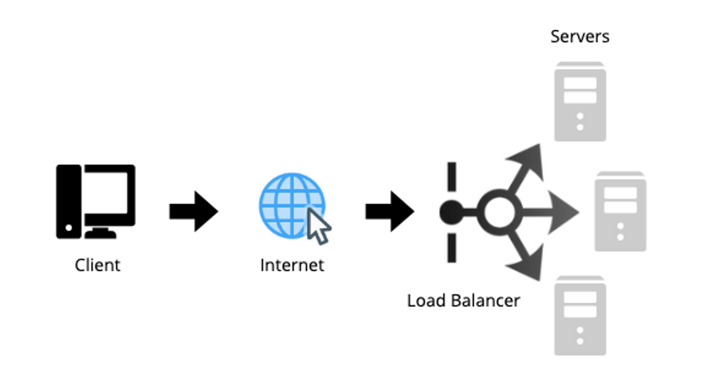
A load balancer is a common, but critical element to any distributed system. Its job is to spread traffic over a cluster of servers to improve the accessibility and responsiveness of apps, web sites or databases. Additionally, a well-designed load balancer can monitor the status of its servers while making requests. For example, a load balancer will quit sending traffic to a server if the server fails a health check, which means it isn’t currently accessible, isn’t responding or has an increased error rate.
Typically, a load balancer will be set between the client and the server, utilizing complex algorithms to route traffic appropriately. The purpose of the algorithms is to maintain a balance on server load across all servers, this will reduce single points of failure in a system, hence improving the systems accessibility and responsiveness.
Here is an image detailing a load balancers place in a simple system:
Since load balancers usually sit between the client and the servers, we can take this knowledge and apply it to other parts of a system. A load balancer can go in many places, some examples are:
- Between the client and server
- Between servers and other internal platform layers, such as, cache or application layers
- Between an internal platform layer and database
While the load balancer’s goal is to reduce a single point of failure, it in itself is a single point of failure in the sense that if the load balancer goes down then it can’t route traffic effectively anymore. To add an extra layer of security, one may choose to add a redundant load balancer in case the original fails, this one maintains all the functionality of the original and is passive. The redundant load balancer will only come into effect once the original has failed.
Why use a load balancer?
- Scalability is a huge benefit since a spike in traffic can be effectively dealt with. Implementing load balancers to handle increased web traffic is easier than moving a site to a more powerful server.
- If implemented successfully, can decrease wait time for users.
- Load balancers can provide unique insight and predictive analytics, most notably helping to spot traffic choke points. This data can factor into business decisions.
- Devices are less stressed since care is taken to distribute work evenly, thus not putting any particular server under undue amounts of stress.
Load Balancing Methods
One of the ways a load balancer decides when to forward requests to its servers is by performing something called a “health check”. These health checks are periodically performed on the backend servers by connection to them, if a server fails a health check” then it will be removed from the group of servers until it is able to connect successfully again.
A health check is one method load balancers use, here are a few more:
- Round Robin - In this method the algorithm cycles through all servers, sending requests to one server and then moving onto the next. This method is simple and works best when the servers all have equal capacity.
- Weighted Round Robin - This method is similar to the round robin method except that it is meant to accommodate servers with differing capacities. Each server in the cluster is assigned a value of some sort (relative to its capacity), servers with higher values receive new connections before the servers with lower values.
- Least Connection - This particular algorithm functions by directing traffic to the server with the least active connections, hence the name. This method works well when connections to all the servers are not evenly distributed.
- Least Response Time - This method directs traffic to the server with the fewest active connections and the lowest average response time.
- Least Bandwidth - The server with the least amount of traffic is selected, traffic is measured by megabits per second (Mbps).
Helpful links on load balancers:
Replication & Redundancy
Redundancy & Replication
Redundancy is a key system design concept, its goal is to remove single points of failure. What redundancy does is duplicate critical system components with the goal of increasing the systems overall reliability. Maintaining backups of critical files or components allows our system to not lose data should the worst come to happen, the loss of data is never ideal and great care should be taken to prevent that.
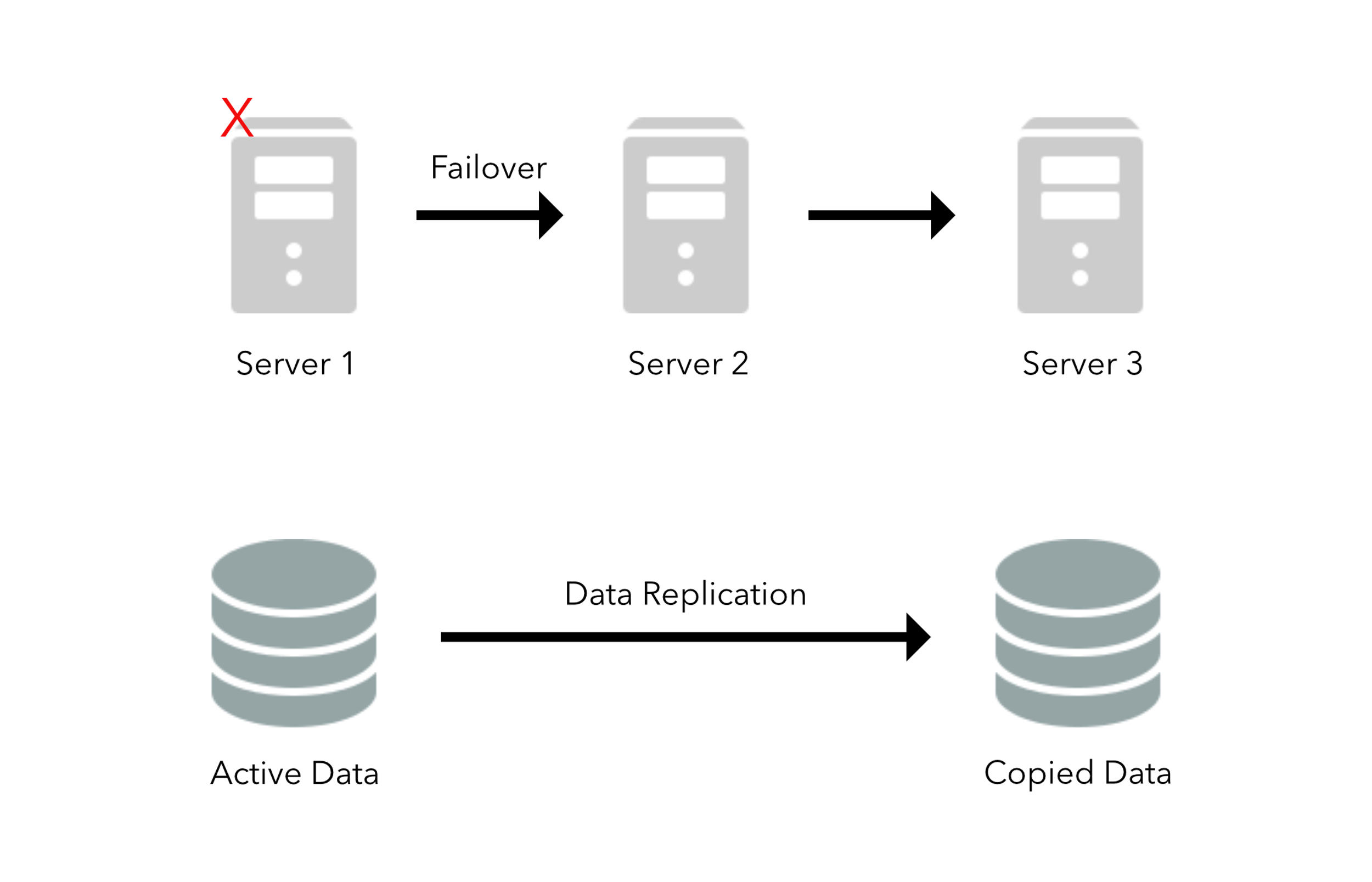
There are two main methods for implementing redundancy in a system, one is active and the other passive .
In a system that uses active redundancy traffic can go to all nodes, in this scenario we usually rely on a load balancer and a method (like round-robin) to distribute traffic amongst all nodes. Since active redundancy involves using multiple nodes, it’s easy to see how this technique is used in scaling systems.
Another option for systems to use is passive redundancy . With this technique the system maintains backup nodes/components to take over in case the main component fails. This is commonly know as master/slave, where one ‘master’ is maintained and whenever the master fails the ‘slaves’ can step in and take over.
Some disadvantages with passive redundancy are the additional complexity it introduces into a system, be it hardware or code. Another downside is the potential for new data to be lost if the system fails before any data can be written to the ‘passive’ node.
Replication is another useful concept, that is very similar to redundancy, since it still involves duplicating nodes. Replication differs because it is more focused on synchronizing data between different nodes, this helps ensure data remains consistent throughout the system even if a few nodes go down. This technique is crucial to maintaining a reliable, accessible and fault-tolerant system.
Replication usually works well with the master/slave technique, as the master can pass data/updates down to all its slaves to ensure data remains consistent.
Helpful links on availability patterns:
SQL vs. NoSQL
SQL vs. NoSQL
When it comes to selecting databases for your system you have two types of solutions to choose from: SQL or NoSQL (Relational database or Non-relational database). While both accomplish the same goal of storing data they go about it in different ways and there are a number of differences, both subtle and pronounced.
One of the key differences right from the bat is that relational databases (SQL) have structure to them, like a predefined schema in which to store data. You can think of relational databases like a phonebook, which stores all the same information for each entry, name, address, phone number. Phonebooks have a structure to them, just like a schema.
Non-relational databases (NoSQL) on the other hand are more dynamic, there is no strict schema that defines data within the database, this can afford the developer more flexibility when designing their data models. An analogy for a non-relational could be a folder that holds a variety of data, such as, text, photos, links and more.
Another difference is that while both database types are capable of horizontal scaling, non-relational databases are popular for being more well-suited for this than relational databases are since it is more time-consuming and expensive…
One last key difference is the difference between ACID and BASE, which relational and non-relational databases are compliant with respectively. ACID compliant databases are more focused on reliability, ensuring transactions are safe and contain the correct data. BASE compliant databases sacrifice some reliability for better performance and scalability.
SQL
In relational databases all data is stored in tables, which are comprised or rows and columns. Each row in the table contains all the information about one entity, while the columns contain the individual data that comprises the aforementioned entity.
For example, let’s say we have an entity in our SQL database that represents a book, a row in the database table is the book entity. Each column displays the relevant info for the book entity, such as name, description, release date, author, price etc…
Popular relational database technologies: MySQL, PostgresSQL, MS SQL Server, Oracle and MariaDB
NoSQL
There are various types on non-relational databases, they have several characteristics like performance, scalability, flexibility and have varying complexity to implement.
Here are a few of the most common types of NoSQL databases:
Key-Value Model - Data stored in this manner is done with key-value pairs. Similar to a hash table, the key is a unique identifier that points to a value.
Examples: Redis, Dynamo and Azure.
Column Store - Otherwise known as a wide-column store, this method uses a concept called a ‘keyspace’ to store column families, which are like containers for rows. Column stores are very dynamic since columns do not need to be known upfront and can have a varying number of columns. Some benefits of a column store is high performance and good scalability.
Examples: HBase, Cassandra
Document Database - Similar to the key-value database, this method stores data in a document which can be queried by referencing its unique key and contains semi-structured data. Data can be stored in many formats like XML, YAML, BSON but the most popular is JSON. One benefit is the ability to query all the data at once, or even small segments of it, this differs from the strictly key-value databases in the fact that queried data retrieves all of it, even if the data is huge.
Document databases are commonly used in blogging platforms, commerce sites and is useful for implementing real-time analytics.
Examples: MongoDB, CouchDB, MarkLogic
Graph Database - In this database type, data is represented as a graph. Graph databases are best used with data that is interconnected, think social networks. The benefits of using this database are that it provides flexibility, since it has no defined schema, data is more fluid and can compile data quicker since it is more localized in the database, as opposed to a normal relational database which could rely on several joins to fetch data from its tables.
Examples: BlazeGraph, OrientDB, Neo4j
Reasons to use SQL database
When it comes to database technology, there’s no one-size-fits-all solution. That’s why many businesses rely on both relational and non-relational databases for different tasks. Even as NoSQL databases gain popularity for their speed and scalability, there are still situations where a highly structured SQL database may be preferable.
Here are a few reasons to choose a SQL database:
-
If you need to ensure ACID compliancy (Atomicity, Consistency, Isolation, Durability). ACID compliancy reduces anomalies and protects the integrity of your database by prescribing exactly how transactions interact with the database. Generally, NoSQL databases sacrifice ACID compliancy for flexibility and processing speed, but for many e-commerce and financial applications, an ACID-compliant database remains the preferred option.
-
Your data is structured and unchanging. If your business is not experiencing massive growth that would require more servers and you’re only working with data that’s consistent, then there may be no reason to use a system designed to support a variety of data types and high traffic volume.
Reasons to use NoSQL database
When all of the other components of your server-side application are designed to be fast and seamless, NoSQL databases prevent data from being the bottleneck. Big data is the real NoSQL motivator here, doing things that traditional relational databases cannot. It’s driving the popularity of NoSQL databases like MongoDB, CouchDB, Cassandra, and HBase.
-
Storing large volumes of data that often have little to no structure. A NoSQL database sets no limits on the types of data you can store together, and allows you to add different new types as your needs change. With document-based databases, you can store data in one place without having to define what “types” of data those are in advance.
-
Making the most of cloud computing and storage. Cloud-based storage is an excellent cost-saving solution, but requires data to be easily spread across multiple servers to scale up. Using commodity (affordable, smaller) hardware on-site or in the cloud saves you the hassle of additional software, and NoSQL databases like Cassandra are designed to be scaled across multiple data centers out of the box without a lot of headaches.
-
Rapid development. NoSQL data doesn’t need to be prepped ahead of time, it is possible to crank out quick iterations, or make frequent updates to the data structure without a lot of downtime between versions, a relational database will slow you down.
Helpful links on SQL vs. NoSQL
https://www.thegeekstuff.com/2014/01/sql-vs-nosql-db
System Design Interviews: A Step By Step Guide
System Design Interviews: A Step By Step Guide
System design interviews (SDIs) are regarded as the hardest portion of the technical interview by most software engineers, primarily because of three reasons:
- Many people struggle because of the open-ended nature of SDI’s, there is no “right” answer only as much as you can justify your solution.
- Lack of experience developing/designing large scale systems in the real world.
- Didn’t prepare enough for SDI’s.
Similar to coding interviews, if candidates do not prepare for SDI’s sufficiently, they will most likely perform poorly. This is made worse if the candidate is interviewing at large companies like, Amazon, Microsoft, Google etc… In these companies, SDI’s are usually more prevalent given the many large scale products these big companies own, performing poorly here can significantly reduce your chance of receiving an offer. Conversely, performing well in an SDI is always a good indicator you might receive an offer (possibly higher position and salary as well).
Step 1: Requirements Clarification
It is crucial in any design interview that you ask questions, the goal being to identify the scope of the problem and clarify ambiguities. Since SDI’s are mostly open-ended, asking the right questions can set you off to a good start and increase your chance of having a successful interview.
For every step, we’ll give examples of different design considerations for developing a service like instagram.
Here are some questions a candidate could ask when designing an instagram-like service:
- Should we design and create a timeline feature?
- Will posts have to accommodate both photo and video?
- Should we the Instagram stories feature?
- Are we designing for both front end and backend?
- Can suers earth hash tags?
- Should users be able to message each other?
- Will there need to be push notifications?
By asking these questions, the candidate is clarifying exactly what he/she needs to build. This defines a plan of action in which you can tackle each step one by one. All these questions determine how the final product will look like.
Step 2: Define API’s
Now that you’ve asked the right questions, you can start defining the API’s you system will use. Going over this with your interviewer will help ensure you haven’t got any of the requirements wrong.
Let’s go over a few examples for our Instagram-like service:
postPhoto(user_id, post_data, user_location, timestamp, …)
updateStory(user_id, post_id, media_upload, timestamp, viewer_count …)
generateFeed(user_id, friend_ids, current_time, …)
likePost(user_id, post_id, …)
These API’s help define what kind of service we’re building, use this to build out a high-level design later on.
Step 3: Scale Estimation
When building any distributed system, it is always a good idea to estimate the scale of the system being designed. Estimation will give you a better idea on where to focus on load balancing, partitioning and caching as you can identify problem areas quicker.
- What scale is expected from the system (e.g., number of new posts, number of post views, how many timeline generations per sec., etc.)?
- How much storage will we need? We will have different numbers if users can have photos and videos in their posts.
- What is the network bandwidth usage we expect? This would be crucial in deciding how would we manage traffic and balance load between servers.
Try to focus your questions on areas that might require a lot of overhead down the line, try to think of certain parts of your design and “stretch” it to its limits and see if that might cause problems if not handled correctly. Storage requirements and requests per second are also huge considerations, especially if you have an app that operates in real-time (ex: Uber).
Step 4: Define Data Model
After defining API’s and scale a candidate should be able to identify the various entities (data models) their system will use, and, more importantly, how the data will be handled and manipulated in respect to the systems requirements. It’s important to consider how your data models will aid in storage, interacting with API’s, encryption and more.
Here are some data models for our Instagram-like service:
User: UserID, Name, Email, DoB, CreationData, LastLogin, etc.
Post: UserID, PostID, PostData, UserLocation, NumberOfLikes, TimeStamp, etc.
Story: UserID, TimeStamp, StoryData
Message: UserID, RecipientID, TimeStamp, MessageData
Timeline: UserID, FollowingID
After defining your data models, you should ask yourself questions like what database should you use? What works best with your data and system overall? NoSQL or MySQL? How can you best store media like photos and videos efficiently.
Step 5: High-Level Design
Discuss with your interviewer as you draw a diagram on about 5-6 components your system design will include. The components don’t need to cover the whole system down to the tiniest detail, but should cover it sufficiently enough to solve the problem at hand. This is the part where we connect our system together and start discussing topics like load balancing, databases, caching etc…
For our Instagram service, at a high level, we will need several components. Here are some requirements:
- We would need a media upload service (for photo and video posts, stories), this will take our media data and upload it to a queue for processing.
- Our service will need multiple application servers to serve all the read/write requests with load balancers in front of them for traffic distributions.
- A distributed file storage will be key for all the photos and videos users will upload. Especially useful since we can archive user stories for reference later in the app.
- We require an efficient database solution to handle all post data for users, needs to be able to support large amounts of read requests.
Remember, this is a high-level design. Your goal is to cover a few of the most important components of your system, and describe to the interviewer how they might work. Establishing your idea at a high-level allows you to dig down deeper into a select few and really give your interviewer a lot of detail.
Step 6: Detailed Design
Dig deeper into 2-3 components; interviewers feedback should always guide you towards which parts of the system he wants you to explain further. You should be able to provide different approaches, their pros and cons, and why would you choose one? Remember there is no single answer, the only important thing is to consider tradeoffs between different options while keeping system constraints in mind.
- Since we will be storing a massive amount of data, how should we partition our data to distribute it to multiple databases? Should we try to store all the data of a user on the same database? What issue can it cause?
- How would we handle “hot” users, who post a lot or follow lots of people?
- Since user’s timeline will contain most recent (and relevant) posts, should we try to store our data in such a way that is optimized to scan latest posts?
- How much and at which layer should we introduce cache to speed things up?
- What components need better load balancing?
Step 7: Identify & Resolve Bottlenecks
Bottlenecks are inevitable in any system, it’s your goal to identify and mitigate/eliminate them from your design. It’s important to bring these up to your interviewer as well as it makes you seem like you understand your system well and possess the foresight to see potential issues in your immediate design. A conscientious engineer is a coveted asset at any company.
Below are some considerations you should have when identifying bottlenecks:
- Is there any single point of failure in our system? What are we doing to mitigate it?
- Do we’ve enough replicas of the data so that if we lose a few servers, we can still serve our users?
- Similarly, do we’ve enough copies of different services running, such that a few failures will not cause total system shutdown?
- How are we monitoring the performance of our service? Do we get alerts whenever critical components fail or their performance degrade?
Summary
During a SDI, if you slow down and remember all the steps laid out in this section, it will help clarify your train of thought, showcase structure to your interviewer and allow you to incrementally build your design better from the ground up. Just remember that practice makes perfect.