s08e39 - 176,113 tech salaries visualized
A big example project - 176,113 tech salaries visualized
We’re going to build this:
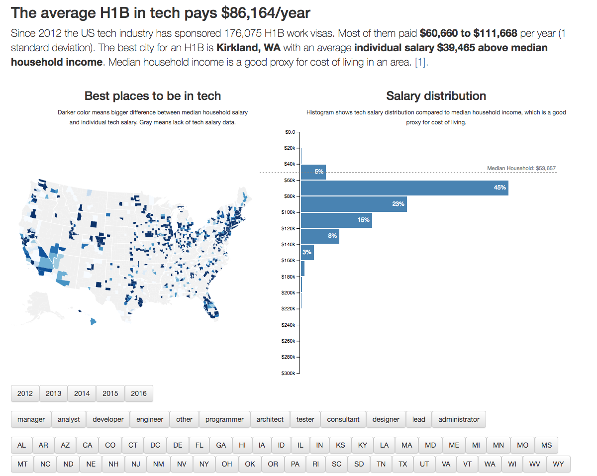
An interactive visualization dashboard app with a choropleth map and a histogram comparing tech salaries to median household income in the area. Users can filter by year, job title, or US state to get a better view.

It’s going to be great.
At this point, I assume you’ve used create-react-app to set up your environment. Check the getting started section if you haven’t. I’m also assuming you’ve read the basics chapter. I’m still going to explain what we’re doing, but knowing the basics helps.
I suggest you follow along, keep npm start running, and watch your visualization change in real time as you code. It’s rewarding as hell.
If you get stuck, you can use my react-d3-walkthrough-livecode to jump between steps. The commits correspond to the code at the end of each step. Check out the first commit and run npm install to skip the initial setup.
If you want to see how this project evolved over 22 months, check the original repo. The modern-code branch has the code you’re about to build.
s09e40 - Show a Preloader
Show a Preloader

Preloader screenshot
Our preloader is a screenshot of the final result. Usually you’d have to wait until the end of the project to make that, but I’ll just give you mine. Starting with the preloader makes sense for two reasons:
- It’s nicer than looking at a blank screen while data loads
- It’s a good sanity check for our environment
We’re using a screenshot of the final result because the full dataset takes a few seconds to load, parse, and render. It looks better if visitors see something informative while they wait.
React Suspense is about to make building preloaders a whole lot better. Adapting to the user’s network speed, built-in preload functionality, stuff like that. More on that in the chapter on React Suspense and Time Slicing.
Make sure you’ve installed all dependencies and that npm start is running.
We’re building our preloader in 4 steps:
- Get the image
- Make the
Preloadercomponent - Update
App - Load Bootstrap styles in
index.js
s09e41 - Step1: get image
Step 1: Get the image
Download my screenshot from Github and save it in src/assets/preloading.png . It goes in the src/assets/ directory because we’re going to import it in JavaScript (which makes it part of our source code), and I like to put non-JavaScript files in assets . Keeps the project organized.
s09e42 - Step 2: make component
Step 2: Preloader component
Our Preloader is a small component that pretends it’s the App and renders a static title, description, and a screenshot of the end result. It goes in src/components/Preloader.js .
We’ll put all of our components in src/components/ .
We start the component off with some imports, an export, and a functional stateless component that returns an empty div element.
// src/components/Preloader.js

import React from "react";

import PreloaderImg from "../assets/preloading.png";

const Preloader = () => (
    <div className="App container">

    </div>
);

export default Preloader;
We import React (which we need to make JSX syntax work) and the PreloaderImg for our image. We can import images because of the Webpack configuration that comes with create-react-app . The webpack image loader returns a URL that we put in the PreloaderImg constant.
At the bottom, we export default Preloader so that we can use it in App.js as import Preloader . Default exports are great when your file exports a single object. Named exports when you want to export multiple items. You’ll see that play out in the rest of this project.
The Preloader function takes no props (because we don’t need any) and returns an empty div . Let’s fill it in.
// src/components/Preloader.js

const Preloader = () => (
    <div className="App container">
        <h1>The average H1B in tech pays $86,164/year</h1>
        <p className="lead">
            Since 2012 the US tech industry has sponsored 176,075 H1B work
            visas. Most of them paid <b>$60,660 to $111,668</b> per year (1
            standard deviation).{" "}
            <span>
                The best city for an H1B is <b>Kirkland, WA</b> with an average
                individual salary <b>$39,465 above local household median</b>.
                Median household salary is a good proxy for cost of living in an
                area.
            </span>
        </p>
        <img
            src={PreloaderImg}
            style={{ width: "100%" }}
            alt="Loading preview"
        />
        <h2 className="text-center">Loading data ...</h2>
    </div>
);
A little cheating with grabbing copy from the future, but that’s okay. In real life you’d use some temporary text, then fill it in later.
The code itself looks like HTML. We have the usual tags - h1 , p , b , img , and h2 . That’s what I like about JSX: it’s familiar. Even if you don’t know React, you can guess what’s going on here.
But look at the img tag: the src attribute is dynamic, defined by PreloaderImg , and the style attribute takes an object, not a string. That’s because JSX is more than HTML; it’s JavaScript. Think of props as function arguments – any valid JavaScript fits.
That will be a cornerstone of our project.
s09e43 - Step 3: Update App
Step 3: Update App
We use our new Preloader component in App – src/App.js . Let’s remove the create-react-app defaults and import our Preloader component.
// src/App.js

import React from 'react';
// Delete the line(s) between here...
import logo from './logo.svg';
import './App.css';
// ...and here.

// Insert the line(s) between here...
import Preloader from './components/Preloader';
// ...and here.

class App extends React.Component {
    // Delete the line(s) between here...
  render() {
    return (
      <div className="App">
        <div className="App-header">
          <img src={logo} className="App-logo" alt="logo" />
          <h2>Welcome to React</h2>
        </div>
        <p className="App-intro">
          To get started, edit <code>src/App.js</code> and save to reload.
        </p>
      </div>
    );
  }
    // ...and here.
}

export default App;
We removed the logo and style imports, added an import for Preloader , and gutted the App class. It’s great for a default app, but we don’t need that anymore.
Let’s define a default state and a render method that uses our Preloader component when there’s no data.
// src/App.js

class App extends React.Component {
    // Insert the line(s) between here...
    state = {
        techSalaries: []
    }

    render() {
        const { techSalaries } = this.state;

        if (techSalaries.length < 1) {
            return (
                <Preloader />
            );
        }

        return (
            <div className="App">

            </div>
        );
    }
    // ...and here.
}
Nowadays we can define properties directly in the class body without a constructor method. It’s not part of the official JavaScript standard yet, but most React codebases use this pattern.
Properties defined this way are bound to each instance of our components so they have the correct this value. Late you’ll see we can use this shorthand to neatly define event handlers.
We set techSalaries to an empty array by default. In render we use object destructuring to take techSalaries out of component state, this.state , and check whether it’s empty. When techSalaries is empty our component renders the preloader, otherwise an empty div.
If your npm start is running, the preloader should show up on your screen.

Preloader without Bootstrap styles
Hmm… that’s not very pretty. Let’s fix it.
s09e44 - Step 4: Load styles
Step 4: Load Bootstrap styles
We’re going to use Bootstrap styles to avoid reinventing the wheel. We’re ignoring their JavaScript widgets and the amazing integration built by the react-bootstrap team. Just the stylesheets please.
They’ll make our fonts look better, help with layouting, and make buttons look like buttons. We could use styled components, but writing our own styles detracts from this tutorial.
We load stylesheets in src/index.js .
// src/index.js

import React from 'react';
import ReactDOM from 'react-dom';
import App from './App';
// Insert the line(s) between here...
import 'bootstrap/dist/css/bootstrap.css';
// ...and here.

ReactDOM.render(
  <App />,
  document.getElementById('root')
);
Another benefit of Webpack: import -ing stylesheets. These imports turn into <style> tags with CSS in their body at runtime.
This is also a good opportunity to see how index.js works to render our app 
- loads
Appand React - loads styles
- Uses
ReactDOMto render<App />into the DOM
That’s it.
Your preloader screen should look better now.
Preloader screenshot
If you don’t, try comparing your changes to this diff on Github.
s10e45 - Asynchronously load data
Asynchronously load data
Great! We have a preloader. Time to load some data.
We’ll use D3’s built-in data loading methods and tie their promises into React’s component lifecycle. You could talk to a REST API in the same way. Neither D3 nor React care what the datasource is.
First, you need some data.
Our dataset comes from a few sources. Tech salaries are from h1bdata.info, median household incomes come from the US census data, and I got US geo map info from Mike Bostock’s github repositories. Some elbow grease and python scripts tied them all together.
You can read about the scraping on my blog here, here, and here. But it’s not the subject of this book.
s10e46 - Step 0: Get data
Step 0: Get the data
Download the data files from my walkthrough repository on Github. Put them in your public/data directory.
s10e47 - Step 1: Prep App.js
Step 1: Prep App.js
Let’s set up our App component first. That way you’ll see results as soon data loading starts to work.
Start by importing our data loading method - loadAllData - and both D3 and Lodash. We’ll need them later.
// src/App.js
import React from 'react';
// Insert the line(s) between here...
import * as d3 from 'd3';
import _ from 'lodash';
// ...and here.

import Preloader from './components/Preloader';
// Insert the line(s) between here...
import { loadAllData } from './DataHandling';
// ...and here.
You already know about default imports. Importing with {} is how we import named exports. That lets us get multiple things from the same file. You’ll see the export side in Step 2.
Don’t worry about the missing DataHandling file. It’s coming soon.
// src/App.js
class App extends React.Component {
    state = {
        techSalaries: [],
        // Insert the line(s) between here...
        medianIncomes: [],
        countyNames: [],
    };

    componentDidMount() {
        loadAllData(data => this.setState(data));
    }
    // ...and here.
We initiate data loading inside the componentDidMount lifecycle hook. It fires when React first mounts our component into the DOM.
I like to tie data loading to component mounts because it means you aren’t making requests you’ll never use. In a bigger app, you’d use Redux, MobX, or similar to decouple loading from rendering. Many reasons why.
To load our data, we call the loadAllData function, then use this.setState in the callback. This updates App ’s state and triggers a re-render, which updates our entire visualization via props.
Yes, it would be better to make loadAllData return a promise instead of expecting a callback. That was giving me trouble for some reason and it doesn’t matter right now anyway.
We also add two more entries to our state : countyNames , and medianIncomes . Defining what’s in your component state in advance makes your code easier to read. People, including you, know what to expect.
Let’s change the render method to show a message when our data finishes loading.
// src/App.js
  render() {
     const { techSalaries } = this.state;

     if (techSalaries.length < 1) {
         return (
             <Preloader />
         );
      }

    return (
        // Delete the line(s) between here...
        <div className="App">
        // ...and here.
        // Insert the line(s) between here...
        <div className="App container">
            <h1>Loaded {techSalaries.length} salaries</h1>
        // ...and here.
        </div>
    );
}
We added a container class to the main <div> and an <h1> tag that shows how many datapoints there are. You can use any valid JavaScript in curly braces {} and JSX will evaluate it. By convention we only use that ability to calculate display values.
You should now get an error overlay.

DataHandling.js not found error overlay
These nice error overlays come with create-react-app and make your code easier to debug. No hunting around in the terminal to see compilation errors.
Let’s build that file and fill it with our data loading logic.
s10e48 - Step 2: Prep data parsing functions
Step 2: Prep data parsing functions
We’re putting data loading logic in a separate file from App.js because it’s a bunch of functions that work together and don’t have much to do with the App component itself.
We start with two imports and four data parsing functions:
-
cleanIncome, which parses each row of household income data -
dateParse, which we use for parsing dates -
cleanSalary, which parses each row of salary data -
cleanUSStateName, which parses US state names
// src/DataHandling.js
import * as d3 from 'd3';
import _ from 'lodash';

const cleanIncome = (d) => ({
    countyName: d['Name'],
    USstate: d['State'],
    medianIncome: Number(d['Median Household Income']),
    lowerBound: Number(d['90% CI Lower Bound']),
    upperBound: Number(d['90% CI Upper Bound'])
});

const dateParse = d3.timeParse("%m/%d/%Y");

const cleanSalary = (d) => {
    if (!d['base salary'] || Number(d['base salary']) > 300000) {
        return null;
    }

    return {employer: d.employer,
            submit_date: dateParse(d['submit date']),
            start_date: dateParse(d['start date']),
            case_status: d['case status'],
            job_title: d['job title'],
            clean_job_title: d['job title'],
            base_salary: Number(d['base salary']),
            city: d['city'],
            USstate: d['state'],
            county: d['county'],
            countyID: d['countyID']
    };
}

const cleanUSStateName = (d) => ({
    code: d.code,
    id: Number(d.id),
    name: d.name
});

const cleanCounty = d => ({
    id: Number(d.id),
    name: name
});
You’ll see those d3 and lodash imports a lot.
Our data parsing functions all follow the same approach: Take a row of data as d , return a dictionary with nicer key names, cast any numbers or dates into appropriate formats. They all start as strings.
Doing all this parsing now, keeps the rest of our codebase clean. Handling data is always messy. You want to contain that mess as much as possible.
s10e49 - Step 3: Load the datasets
Step 3: Load the datasets
Now we can use D3 to load our data with fetch requests.
// src/DataHandling.js
export const loadAllData = (callback = _.noop) => {
    Promise.all([
        d3.json("data/us.json"),
        d3.csv("data/us-county-names-normalized.csv", cleanCounty),
        d3.csv("data/county-median-incomes.csv", cleanIncome),
        d3.csv("data/h1bs-2012-2016-shortened.csv", cleanSalary),
        d3.tsv("data/us-state-names.tsv", cleanUSStateName)
    ]).then(([us, countyNames, medianIncomes, techSalaries, USstateNames]) => {

    });
};
Here you can see another ES6 trick: default argument values. If callback is undefined, we set it to _.noop - a function that does nothing. This lets us later call callback() without worrying whether it’s defined.
In version 5, D3 updated its data loading methods to use promises instead of callbacks. You can load a single file using d3.csv("filename"😉.then(data => .... . The promise resolves with your data, or throws an error.
If you’re on D3v4 and can’t upgrade, you’ll have to import from d3-fetch .
Each d3.csv call makes a fetch request, parses the fetched CSV file into an array of JavaScript dictionaries, and passes each row through the provided cleanup function. We pass all median incomes through cleanIncome , salaries through cleanSalary , etc.
To load multiple files, we use Promise.all with a list of unresolved promises. Once resolved, our .then handler gets a list of results. We use array destructuring to expand that list into our respective datasets before running some more logic to tie them together.
D3 supports formats like json , csv , tsv , text , and xml out of the box. You can make it work with custom data sources through the underlying request API.
PS: we’re using the shortened salary dataset to make page reloads faster while building our project.
s10e50 - Step 4: Tie datasets together
Step 4: Tie the datasets together
If you add a console.log to the .then callback above, you’ll see a bunch of data. Each argument - us , countyNames , medianIncomes , techSalaries , USstateNames - holds a parsed dataset from the corresponding file.
To tie them together and prepare a dictionary for setState back in the App component, we need to add some logic. We’re building a dictionary of county household incomes and removing any empty salaries.
// src/DataHandling.js
]).then(([us, countyNames, medianIncomes, techSalaries, USstateNames]) => {
    let medianIncomesMap = {};

    medianIncomes.filter(d => _.find(countyNames,
                                     {name: d['countyName']}))
                 .forEach((d) => {
                     d['countyID'] = _.find(countyNames,
                                            {name: d['countyName']}).id;
                     medianIncomesMap[d.countyID] = d;
                 });

    techSalaries = techSalaries.filter(d => !_.isNull(d));

    callback({
        usTopoJson: us,
        countyNames: countyNames,
        medianIncomes: medianIncomesMap,
        medianIncomesByCounty: _.groupBy(medianIncomes, 'countyName'),
        medianIncomesByUSState: _.groupBy(medianIncomes, 'USstate'),
        techSalaries: techSalaries,
        USstateNames: USstateNames
    });
});
Building the income map looks weird because of indentation, but it’s not that bad. We filter the medianIncomes array to discard any incomes whose countyName we can’t find. I made sure they were all unique when I built the datasets.
We walk through the filtered array with a forEach , find the correct countyID , and add each entry to medianIncomesMap . When we’re done, we have a large dictionary that maps county ids to their household income data.
Then we filter techSalaries to remove any empty values where the cleanSalaries function returned null . That happens when a salary is either undefined or absurdly high.
When our data is ready, we call our callback with a dictionary of the new datasets. To make future access quicker, we use _.groupBy to build dictionary maps of counties by county name and by US state.
You should now see how many salary entries the shortened dataset contains.

Data loaded screenshot
If that didn’t work, try comparing your changes to this diff on Github.
s11e51 - Render a choropleth map of the US
Render a choropleth map of the US
With our data in hand, it’s time to draw some pictures. A choropleth map will show us the best places to be in tech.
We’re showing the delta between median household salary in a statistical county and the average salary of an individual tech worker on a visa. The darker the blue, the higher the difference.
The more a single salary can out-earn an entire household, the better off you are.
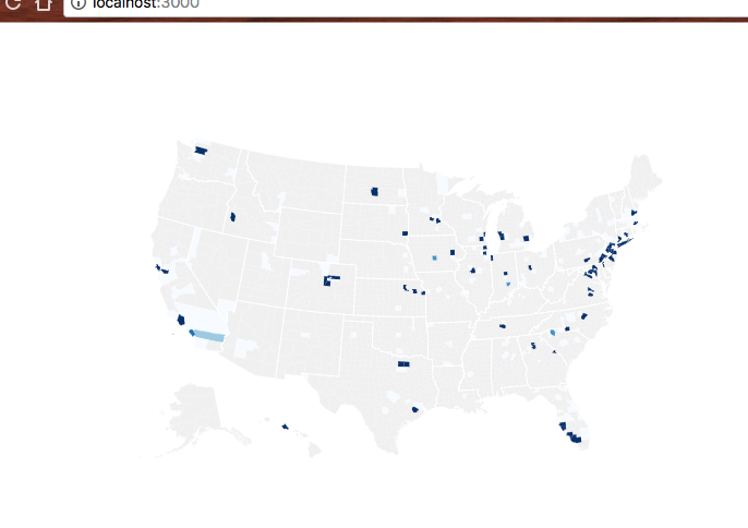
Choropleth map with shortened dataset
There’s a lot of gray on this map because the shortened dataset doesn’t have that many counties. Full dataset is going to look better, I promise.
Turns out immigration visa opportunities for techies aren’t evenly distributed throughout the country. Who knew?
Just like before, we’re going to start with changes in our App component, then build the new bit. This time, a CountyMap component spread over three files:
-
CountyMap/index.js, to make imports easier -
CountyMap/CountyMap.js, for overall map logic -
CountyMap/County.js, for individual county polygons
s11e52 - Step 1: Prep App.js
Step 1: Prep App.js
You might guess the pattern already: add an import, add a helper method or two, update render .
// src/App.js
import Preloader from './components/Preloader';
import { loadAllData } from './DataHandling';

// Insert the line(s) between here...
import CountyMap from './components/CountyMap';
// ...and here.
That imports the CountyMap component from components/CountyMap/ . Your browser will show an error overlay about some file or another until we’re done.
In the App class itself, we add a countyValue method. It takes a county entry and a map of tech salaries, and it returns the delta between median household income and a single tech salary.
    // src/App.js
    countyValue(county, techSalariesMap) {
        const medianHousehold = this.state.medianIncomes[county.id],
              salaries = techSalariesMap[county.name];

        if (!medianHousehold || !salaries) {
            return null;
        }

        const median = d3.median(salaries, d => d.base_salary);

        return {
            countyID: county.id,
            value: median - medianHousehold.medianIncome
        };
    }
We use this.state.medianIncomes to get the median household salary and the techSalariesMap input to get salaries for a specific census area. Then we use d3.median to calculate the median value for salaries and return a two-element dictionary with the result.
countyID specifies the county and value is the delta that our choropleth displays.
In the render method, we’ll:
- prep a list of county values
- remove the “data loaded” indicator
- render the map
// src/App.js
render() {
    // Insert the line(s) between here...
    const { countyNames, usTopoJson, techSalaries, } = this.state;
    // ...and here.

    if (techSalaries.length < 1) {
        return (
            <Preloader />
        );
    }

    // Insert the line(s) between here...
    const filteredSalaries = techSalaries,
          filteredSalariesMap = _.groupBy(filteredSalaries, 'countyID'),
          countyValues = countyNames.map(
              county => this.countyValue(county, filteredSalariesMap)
          ).filter(d => !_.isNull(d));

    let zoom = null;
    // ...and here.

    return (
      <div className="App container">
        // Delete the line(s) between here...
        <h1>Loaded {techSalaries.length} salaries</h1>
        // ...and here.
        // Insert the line(s) between here...
        <svg width="1100" height="500">
            <CountyMap usTopoJson={usTopoJson}
                       USstateNames={USstateNames}
                       values={countyValues}
                       x={0}
                       y={0}
                       width={500}
                       height={500}
                       zoom={zoom} />
        </svg>
        // ...and here.
      </div>
    );
}
We call our dataset filteredTechSalaries because we’re going to add filtering in the subchapter about adding user controls. Using the proper name now means less code to change later. The magic of foresight 
We use _.groupBy to build a dictionary mapping each countyID to an array of salaries, and we use our countyValue method to build an array of counties for our map.
We set zoom to null for now. We’ll use this later.
In the return statement, we remove our “data loaded” indicator, and add an <svg> element that’s 1100 pixels wide and 500 pixels high. Inside, we place the CountyMap component with a bunch of properties. Some dataset stuff, some sizing and positioning stuff.
s11e53 - Step 2: CountyMap index.js
Step 2: CountyMap/index.js
We make index.js for just reason: to make imports and debugging easier. I learned this lesson the hard way so you don’t have to.
// src/components/CountyMap/index.js

export { default } from './CountyMap';
Re-export the default import from ./CountyMap.js . That’s it.
This allows us to import CountyMap from the directory without knowing about internal file structure. We could put all the code in this index.js file, but that makes debugging harder. You’ll have plenty of index.js files in your project.
Having a lot of code in <directory>/index.js is a common pattern in new projects. But when you’re looking at a stack trace, source files in the browser, or filenames in your editor, you’ll wish every component lived in a file of the same name.
s11e54 - Step 3: CountyMap CountyMap.js
Step 3: CountyMap/CountyMap.js
Here comes the fun part - declaratively drawing a map. You’ll see why I love using React for dataviz.
We’re using the full-feature integration approach and a lot of D3 maps magic. Drawing a map with D3 I’m always surprised how little code it takes.
Start with the imports: React, D3, lodash, topojson, County component.
// src/components/CountyMap/CountyMap.js
import React, { Component } from 'react';
import * as d3 from 'd3';
import * as topojson from 'topojson';
import _ from 'lodash';

import County from './County';
Out of these, we haven’t built County yet, and you haven’t seen topojson before.
TopoJSON is a geographical data format based on JSON. We’re using the topojson library to translate our geographical datasets into GeoJSON, which is another way of defining geo data with JSON.
I don’t know why there are two, but TopoJSON produces smaller files, and GeoJSON can be fed directly into D3’s geo functions. ¯\ (ツ) /¯
Maybe it’s a case of competing standards.
Constructor
We stub out the CountyMap component then fill it in with logic.
// src/components/CountyMap/CountyMap.js
class CountyMap extends Component {
    constructor(props) {
        super(props);

        this.state = {
        }
    }

    static getDerivedStateFromProps(props, state) {

    }

    render() {
        const { usTopoJson } = this.props;

        if (!usTopoJson) {
            return null;
        }else{
            return (

            );
        }
    }
}

export default CountyMap;
We’ll set up default D3 state in constructor and keep it up to date with getDerivedStateFromProps .
We need three D3 objects to build a choropleth map: a geographical projection, a path generator, and a quantize scale for colors.
// src/components/CountyMap/CountyMap.js
class CountyMap extends React.Component {
    constructor(props) {
        super(props);

        const projection = d3.geoAlbersUsa().scale(1280);

        this.state = {
            geoPath: d3.geoPath().projection(projection),
            quantize: d3.scaleQuantize().range(d3.range(9)),
            projection
        };
    }
You might remember geographical projections from high school. They map a sphere to a flat surface. We use geoAlbersUsa because it’s made specifically for maps of the USA.
D3 offers many other projections. You can see them on d3-geo’s Github page.
A geoPath generator takes a projection and returns a function that generates the d attribute of <path> elements. This is the most general way to specify SVG shapes. I won’t go into explaining the d here, but it’s an entire language for describing shapes.
quantize is a D3 scale. We’ve talked about the basics of scales in the D3 Axis example. This one splits a domain into 9 quantiles and assigns them specific values from the range .
Let’s say our domain goes from 0 to 90. Calling the scale with any number between 0 and 9 would return 1. 10 to 19 returns 2 and so on. We’ll use it to pick colors from an array.
getDerivedStateFromProps
Keeping our geo path and quantize scale up to date is simple, but we’ll make it harder by adding a zoom feature. It won’t work until we build the filtering, but hey, we’ll already have it by then!
    // src/components/CountyMap/CountyMap.js
    static getDerivedStateFromProps(props, state) {
        let { projection, quantize, geoPath } = state;

        projection
            .translate([props.width / 2, props.height / 2])
            .scale(props.width * 1.3);

        if (props.zoom && props.usTopoJson) {
            const us = props.usTopoJson,
                USstatePaths = topojson.feature(us, us.objects.states).features,
                id = _.find(props.USstateNames, { code: props.zoom }).id;

            projection.scale(props.width * 4.5);

            const centroid = geoPath.centroid(_.find(USstatePaths, { id: id })),
                translate = projection.translate();

            projection.translate([
                translate[0] - centroid[0] + props.width / 2,
                translate[1] - centroid[1] + props.height / 2
            ]);
        }

        if (props.values) {
            quantize.domain([
                d3.quantile(props.values, 0.15, d => d.value),
                d3.quantile(props.values, 0.85, d => d.value)
            ]);
        }

        return {
            ...state,
            projection,
            quantize
        };
    }
There’s a lot going on here.
We destructure projection , quantize , and geoPath out of component state. These are the D3 object we’re about to update.
First up is the projection. We translate (move) it to the center of our drawing area and set the scale property. You have to play around with this value until you get a nice result because it’s different for every projection.
Then we do some weird stuff if zoom is defined.
We get the list of all US state features in our geo data, find the one we’re zoom -ing on, and use the geoPath.centroid method to calculate its center point. This gives us a new coordinate to translate our projection onto.
The calculation in .translate() helps us align the center point of our zoom US state with the center of the drawing area.
While all of this is going on, we also tweak the .scale property to make the map bigger. This creates a zooming effect.
After all that, we update the quantize scale’s domain with new values. Using d3.quantile lets us offset the scale to produce a more interesting map. Again, I discovered these values through experiment - they cut off the top and bottom of the range because there isn’t much there. This brings higher contrast to the richer middle of the range.
With our D3 objects updated, we return a new derived state. Technically you don’t have to do this but you should. Due to how JavaScript works, you already updated D3 objects in place, but you should pretend this.state is immutable and return a new copy.
Overall that makes your code easier to understand and closer to React principles.
render
After all that hard work, the render method is a breeze. We prep our data then loop through it and render a County element for each entry.
    render() {
        const { geoPath, quantize } = this.state,
            { usTopoJson, values, zoom } = this.props;

        if (!usTopoJson) {
            return null;
        } else {
            const us = usTopoJson,
                USstatesMesh = topojson.mesh(
                    us,
                    us.objects.states,
                    (a, b) => a !== b
                ),
                counties = topojson.feature(us, us.objects.counties).features;

            const countyValueMap = _.fromPairs(
                values.map(d => [d.countyID, d.value])
            );

            return (
                <g>
                    {counties.map(feature => (
                        <County
                            geoPath={geoPath}
                            feature={feature}
                            zoom={zoom}
                            key={feature.id}
                            quantize={quantize}
                            value={countyValueMap[feature.id]}
                        />
                    ))}

                    <path
                        d={geoPath(USstatesMesh)}
                        style={{
                            fill: "none",
                            stroke: "#fff",
                            strokeLinejoin: "round"
                        }}
                    />
                </g>
            );
        }
    }
We use destructuring to save all relevant props and state in constants, then use the TopoJSON library to grab data out of the usTopoJson dataset.
.mesh calculates a mesh for US states – a thin line around the edges. .feature calculates feature for each count – fill in with color.
Mesh and feature aren’t tied to US states or counties by the way. It’s just a matter of what you get back: borders or flat areas. What you need depends on what you’re building.
We use Lodash’s _.fromPairs to build a dictionary that maps county identifiers to their values. Building it beforehand makes our code faster. You can read some details about the speed optimizations here.
As promised, the return statement loops through the list of counties and renders County components. Each gets a bunch of attributes and returns a <path> element that looks like a specific county.
For US state borders, we render a single <path> element and use geoPath to generate the d attribute.
s11e55 - Step 4: CountyMap County.js
Step 4: CountyMap/County.js
The County component is built from two parts: imports and color constants, and a component that returns a <path> . All the hard calculation happens in CountyMap .
// src/components/CountyMap/County.js
import React, { Component } from 'react';
import _ from 'lodash';

const ChoroplethColors = _.reverse([
    'rgb(247,251,255)',
    'rgb(222,235,247)',
    'rgb(198,219,239)',
    'rgb(158,202,225)',
    'rgb(107,174,214)',
    'rgb(66,146,198)',
    'rgb(33,113,181)',
    'rgb(8,81,156)',
    'rgb(8,48,107)'
]);

const BlankColor = 'rgb(240,240,240)'
We import React and Lodash, and define some color constants. I got the ChoroplethColors from some example online, and BlankColor is a pleasant gray.
Now we need the County component.
// src/components/CountyMap/County.js
class County extends Component {
    shouldComponentUpdate(nextProps, nextState) {
        const { zoom, value } = this.props;

        return zoom !== nextProps.zoom
            || value !== nextProps.value;
    }

    render() {
        const { value, geoPath, feature, quantize } = this.props;

        let color = BlankColor;

        if (value) {
            color = ChoroplethColors[quantize(value)];
        }

        return (
            <path d={geoPath(feature)}
                  style={{fill: color}}
                  title={feature.id} />
        );
    }
}

export default County;
The render method uses a quantize scale to pick the right color and returns a <path> element. geoPath generates the d attribute, we set style to fill the color, and we give our path a title .
shouldComponentUpdate is more interesting. It’s a React lifecycle method that lets you specify which prop changes are relevant to component re-rendering.
CountyMap passes complex props - quantize , geoPath , and feature . They’re pass-by-reference instead of pass-by-value. That means React can’t see when their output changes unless you make completely new copies.
This can lead to all 3,220 counties re-rendering every time a user does anything. But they only have to re-render if we change the map zoom or if the county gets a new value.
Using shouldComponentUpdate like this we can go from 3,220 DOM updates to a few hundred. Big speed improvement
s11e56 - A map appears 
Your browser should now show a map.
Choropleth map with shortened dataset
Tech work visas just aren’t that evenly distributed. Even with the full dataset most counties are gray.
If that didn’t work, consult this diff on Github.