The Excel Bootcamp: Zero to Mastery / materials

Andrew.Kaluba · 18.Январь.2022 23:01:34

Exercise: Excel 101

“I’ll show these people what you don’t want them to see. A world without rules and controls, without borders or boundaries. A world where anything is possible.” - Neo (The Matrix, 1999)

If you haven’t seen The Matrix film, Neo’s quote here is when he first awakens from the machine world and starts teaching the other humans the basics of how to use Excel (Excel 101). And I agree with him: with Excel anything is possible.

On a more serious note, welcome to our first exercise! You’ll see exercises sprinkled throughout this course, and I highly recommend you do them - exercises are the key to solidifying your understanding of the concepts. And besides, doing is the most fun part of learning!

Of course, if you have any questions or get stuck, hop on over to the #excel channel in ZTM Discord server (invite link available in the “Join The Community” lesson) where I’ll be hanging out to answer any questions you may have.

*All files referenced in exercises are available to download directly below.

Exercise: Excel 101

Download and open the “Customer Reviews.xlsx” file directly below (at the bottom of this page).
Create a new worksheet - positioned to the left of the other worksheet in the file - named “08-12-2021”.
Download and open the “Customer Reviews 08-12-2021.xlsx” file below.
Copy and paste the data in the “Customer Reviews 08-12-2021.xlsx” file into cell A1 of the “Customer Reviews.xlsx” file.
Delete the “ProductID” column in the data.
Unmerge the two cells composing the “CustomerName” column header, and then add “Customer First Name” and “Customer Last Name” headers for the two columns.
Cut the “Customer First Name” and “Customer Last Name” columns, and insert them to the left of the “ReviewStars” column.
Edit the remaining column headers to have spaces between the words in the names (i.e, “ProductName” becomes “Product Name”).
Insert a new column, to the left of the other columns, and give it a column header of “Review Number”.
Using Excel’s autofill feature, populate this column with a series of numbers from one to the number of reviews in the dataset.
Re-format the “Purchase Date” and “Review Date” columns to the MM/DD/YYYY date format.
Re-format the “Review Stars” column to display zero digits after the decimal place.
Using Excel’s find and replace feature, replace all instances of the word “ukelele” on the worksheet with “ukulele”.
Change the font of all the cells in the range to “Segoe UI”, size 10.
Give the column headers a dark background fill color from one of Excel’s built-in “theme” colors - your choice!
Change the font color of the column headers to white.
Bold the column headers.
Auto-fit the widths of the columns to adjust to the width of the data they contain.
Freeze the top row of the data (the column headers) so that it remains visible no matter how far you scroll down through the data.
Save the file AS “Customer Reviews - Formatted.xlsx”.

Solution: your solution should look very similar to the data on the “08-11-2021” worksheet of the “Customer Reviews.xlsx” file. Is it the same? Yes? Great job! No? Hop over to the #excel channel in the ZTM Discord server and I’ll help you figure out what went wrong.

Exercise: Filtering and Sorting Data

“Remember, all I’m offering is the truth. Nothing more." - Morpheus (The Matrix, 1999)

In the movie, Morpheus says this quote to Neo while teaching him how to filter and sort data in Excel. True story!

Here’s your next exercise. This one should be a piece of cake for you but remember - practice, practice, practice!

Exercise: Filtering and Sorting Data

Download and open the “Filtering and Sorting - Starter.xlsx” file below (at the bottom of this page).
Apply filters to the dataset.
Auto-fit column widths if needed.
Filter the “Review Stars” column to only display reviews below 5 stars.
Filter the “Purchase Date” column to only include purchases from August.
Filter the “Product Name” column to only include products that contain the word “board”.
Sort the filtered dataset by “Purchase Date” (newest to oldest), THEN by “Review Stars” (lowest to highest).

Solution: Check your results against the “Filtering and Sorting - Exercise Solution.xlsx” file below. Is it the same? Yes? Great job! No? Hop over to the #excel channel in the ZTM Discord server and I’ll help you figure out what went wrong.

Exercise: Formulas 101

Formulas are where the magic starts to happen, where you can really start doing some wizardry with data. Use this exercise to practice your formulas.

Exercise: Excel Formulas 101

Download and open the “Excel Formulas - Starter.xlsx” file directly below (at the bottom of this page).
On the “Exercise 1” worksheet , insert a blank column to the left of the “Product Name” column, and give it the column header “Days Since Purchase”.
Populate this new column with a formula that calculates the elapsed days between the purchase date and the review date. Make sure the results are formatted as numbers, with 0 digits after the decimal.
Add a new column to the right of “Customer Last Name”, with the column header “Username”.
Populate this column with a formula that automatically generates customer usernames as follows: it should concatenate the customer’s first name, then a period/dot, then the customer’s last name, in a single string.
On the " Exercise 2" worksheet , fill out the multiplication table by writing a single formula in the top left blank cell of the table, then copying that formula over the rest of the table. Each cell in the table should yield the result of multiplying the column header for that cell by its row header.
You will need to employ some combination of absolute and relative cell references in your formula to accomplish this. You can preview what the solution would look like (with no formulas of course!) on the “Multiplication Table Example” worksheet.

Solution : download the “Excel Formulas - Exercise Solution.xlsx” file to check your work.

Exercise: Crunching Numbers With Excel Functions

Just like going to the gym, you need to practice and be consistent to see results. Keep going, you got this!

Exercise: Crunching Numbers With Excel Functions

Download and open the “Home Sale Data.xlsx” file, found in the resources for this section. Review the data on the “Home Sale Data” worksheet , which lists all the homes sold by a particular real estate agency in 2020.
In column B of the “Summary Statistics” worksheet , use built-in Excel functions to calculate the four summary statistics listed in column A.
Insert a blank column to the right of the “AskingPrice” column on the “Home Sale Data” worksheet . Give this column the header “AskingPriceRounded”.
Using a built-in Excel function, populate this new column with the asking prices from the neighboring column, but rounded to zero decimal places.
Insert a blank column to the right of the “SalePrice” column on the “Home Sale Data” worksheet . Give this column the header “SalePriceTruncated”.
Using a built-in Excel function, populate this new column with the sale prices from the neighboring column, but with all digits after the decimal removed (NOT rounded).
Note the difference in how the two approaches handle decimals greater than or equal to 0.5.

Solution: check your results against the "Crunching Numbers With Excel Functions - Exercise Solutions.xlsx"

Exercise: Conditional Calculations

This exercise is a two-parter. Double the fun (and double the skill-building)!

Exercise: Conditional Calculations

Part 1:

Download and open the “Home Sale Data.xlsx” file , found in the resources for this section. Review the data on the “Home Sale Data” worksheet , which lists all the homes sold by a particular real estate agency in 2020.
Using the Ctrl + Shift + Down Arrow keyboard shortcut, select all the agent names from the “Agent” column, then copy and paste these names into cell A2 of the “Exercise 1” worksheet .
Using Excel’s “Remove Duplicates” feature, transform this list of names into just the distinct/unique agent names (there should be 12).
Using Excel’s SUMIFS function, calculate the total 2020 sales by each real estate agent in the “Total 2020 Sales” column on the “Exercise 1” worksheet .

Part 2:

Using the Ctrl + Shift + Down Arrow keyboard shortcut, select all the city names from the “City” column of the “Home Sale Data” worksheet , then copy and paste these cities into cell A2 of the “Exercise 2” worksheet.
Using Excel’s “Remove Duplicates” feature, transform this list of cities into just the distinct/unique agent names (there should be 11).
In columns B through D of the “Exercise 2” worksheet , use Excel’s COUNTIFS function to calculate the total sales for each city in 2020, per the sale price threshold specified in each column header. For example, in column B, you’ll only want to count home sales for the given city in column A, if the sale price was less than $500,000. HINT: you will need to apply multiple criteria in your COUNTIFS functions to get this to work.

Solutions: see the Exercise Solutions file below.

Exercise: Date and Time Functions

This exercise is actually SIX mini-exercises. But by the end of it you’ll be a whiz with the DATE and TIME functions. Rock on!

Exercises: Date & Time Functions

Open and download the “Date and Time Functions - Exercises.xlsx” file below. All these exercises are in worksheets within this file.

Exercise 1

In the “Exercise 1” worksheet of the exercise file, we have a list of product IDs, along with their date of purchase and the length of the product warranty in months. Using the DATE function (in conjunction with YEAR, MONTH, and DAY), calculate the expiration data of the warranty as an offset from the purchase date.

Exercise 2

In the “Exercise 2” worksheet of the exercise file, we have a list of customer order IDs, along with their respective order date/times and the number of hours the orders are required to be processed in (Fulfillment SLA). Using the TIME function (in conjunction with HOUR, MINUTE, and SECOND), calculate when the orders are due to be shipped as an offset from the order date/time.

Exercise 3

Our starter data for Exercise 3 is almost identical to that for exercise 2, with the exception that our order time now has a date component.

In column E, use “date math” to add the value in the “Fulfillment SLA” column to the “Order Datetime” value, to calculate when the orders are due to be shipped.

HINT: Excel looks at time values as simply fractions of a 24 hour day - for example, 12 hours is interpreted as 0.5, since it is half of a 24 hour day. As such, you’ll need to divide the “Fulfillment SLA” by the appropriate number, and then add the result to the Order Datetime.

Exercise 4

For Exercise 4, calculate your age in months using Excel’s DATEDIF function.

Exercise 5

In column F of the “Exercise 5” worksheet , use the NETWORKDAYS function to calculate the number of business days (that is to say, excluding weekends and holidays) elapsed between the Order Datetime in column B and the Delivery Date in column E. You can create a list of holidays observed in your country or place of business, to reference in your function, in the “Holidays” worksheet of the exercise file.

Exercise 6

In column C of the “Exercise 6” worksheet , remove the time component of the datetime values in column B using the TRUNC function.

Then, using the TEXT function, extract the weekday NAME (for example, “Monday”) from the dates into column D.

Exercise: Text Functions

By now you know the drill - download and open the “Text Functions - Exercises.xlsx” file at the bottom of this page to do this exercise!

Exercises: Text Functions

Exercise 1

Using the first and last names provided in the “Exercise 1” worksheet , derive a nickname for each person as follows: the first character of their first name, then a hyphen ("-"), and finally the first three characters of their last name. The entire nickname should be capitalized.

The LEFT and UPPER functions should help you here. Also recall that you can combine multiple text values together with the ampersand ("&") operator.

Exercise 2

Using LEFT/MID/RIGHT - in conjunction with the FIND function - parse out the first, middle, and last names from the list of names in column A of the “Exercise 2” worksheet .

Note that the names have been entered in the following format: “last, first middle”.

Exercise 3

The phone numbers in column A of the “Exercise 3” worksheet have a couple of problems.

First, there is a space before and after each phone number.

Second, some phone numbers have a lowercase letter “o” in place of a zero in the actual phone number.

Clean up these phone numbers using the TRIM and SUBSTITUTE functions.

Exercise: Logical and Lookup Functions

Now we’re cookin’ with Logical and Lookup functions! If you need some inspiration, here’s a quote to get you going: “It’s what we do in the shadows, that puts us in the light”.

Exercises: Logical and Lookup Functions

Open and download the “Logical and Lookup Functions - Exercises.xlsx” file below.

Exercise 1

In column G of the “Exercise 1” worksheet , write an IF formula that returns “Fail” if the actual shipping time in column F is greater than the order delivery goal in column D, and “Pass” otherwise.

Exercise 2

On the “Exercise 2” worksheet , add another layer to your IF formula from the previous exercise as follows:

If the actual shipping time is equal to the order delivery goal, return “Meets”.
If the actual shipping time is greater than the order delivery goal, return “Fail”.
Otherwise (if the actual shipping time is less than the order delivery goal), return “Exceeds”.

Hint: Try using a nested IF function.

Exercise 3

In column G of the “Exercise 3” worksheet , calculate whether or not we need to provide a customer refund based on the following logic:

If the order is a “rush” order (value of “Yes” in column C), AND the actual shipping time is greater than the order delivery goal, return “Yes”.
Otherwise, return “No”.

Hint: Try nesting an “AND” function inside your IF function.

Exercise 4

For the customer names in column A of the “Exercise 4” worksheet , pull in the values for phone number, order date, order amount, and order quantity from the table on the “Customer Data” worksheet .

If no match can be found on the “Customer Data” worksheet , return a user-friendly message like “Not found”.

Exercise 5

For the phone numbers in column A of the “Exercise 5” worksheet , pull in the values for customer name, order date, order amount, and order quantity from the table on the “Customer Data” worksheet .

If no match can be found on the “Customer Data” worksheet , return a user-friendly message like “Not found”.

Hint: The columns on the "Customer Data" worksheet are NOT in the order needed to pull in customer name based on phone number. You’ll need to reorder the columns (try using cut/insert) to get a VLOOKUP function to work for all the values. To keep your Exercise 4 formulas from breaking, I’d suggest making a copy of the “Customer Data” worksheet and then using the copied sheet for Exercise 5.

Exercise: Modeling

Here’s where you get to model! No not a fashion model (although I’ve no doubt that you’re a super good looking person!) but modeling in Excel. This is where the magic really happens!

Exercise: Modeling in Excel

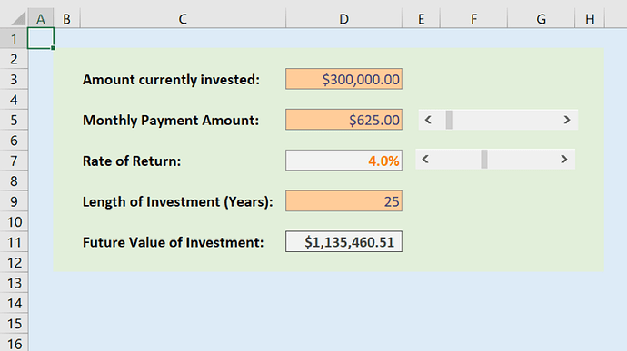
The “Modeling in Excel - Exercise Starter.xlsx” file at the bottom of this page contains a basic model that calculates the future value of an investment (like a retirement plan) based on the following inputs:

The current value of the investment (the input in cell B1)
The monthly payment/contribution to the investment (the input in cell B3)
The rate of return on the investment (the input in cell B5)
The time horizon of the investment (the input in cell B7)

The model uses Excel’s FV (future value) function in cell B9 to calculate the future value of the investment based on the above inputs. You don’t need to understand exactly how the function works (although feel free to inspect it!); our focus in this exercise will be on varying the inputs to the final calculation in a dynamic and systematic way.

Try modifying the model in the starter file to resemble the screenshot below (and if you need it there are specific, step-by-step instructions right below the screenshot):

Set up a scroll bar to vary the monthly payment input between $0 and $10,000.
Set up a scroll bar to vary the rate of return input between 0% and 10%. Remember, rate of return will be a fractional number between 0 and 0.1, and the scroll bar can only handle whole numbers, so you may need to use a formula to translate the linked cell value into a percent.
Use a data validation list to give users of our model the following options for length of investment in years: 5, 10, 15, 20, 25, and 30.
Apply named ranges to all inputs in the model (as well as the range of values used for the data validation list).
Update the FV formula to reference these named ranges instead of cell references.
Use Excel’s built-in cell styles to style the inputs/outputs/calculations of the model appropriately.
Apply any other formatting you deem appropriate to make the model more usable/readable.

Exercise: Data Visualization

DATA. VISUALIZATION. You are visualizing the data, obviously. But think about what this means - it means you can take complex data and display it in a way that someone else (your boss, your friend, your partner) can understand at a glance. Pretty cool if you ask me!

Exercise: Data Visualization in Excel

Download and open the “Data Visualization Exercise Starter.xlsx” file below.

Exercise 1

On the “Home Sale Data” worksheet , apply a conditional formatting rule to the “Acreage” column, such that homes with more than 20 acres are called out. The exact formatting used is up to you.

Exercise 2

On the “Exercise 2” worksheet , apply data bars to the “Total 2020 Sales” column, to give some scale to the numbers. The color/gradient of the bars is up to you.

Exercise 3

Insert a blank column to the right of the “SaleDate” column on the “Home Sale Data” worksheet . Name the column “SaleMonth”.
Populate this column with a formula that returns the name of the month in which the home was sold. For example, if a home was sold on 8/6/2021, this column should have the value “August” for that row. HINT : The TEXT function, with a second argument of “mmmm”, can help here.
On the “Exercise 3” worksheet , use the SUMIFS function to populate the three blank columns with each respective region’s (West, Central, and North) sales for each month. HINT : You will need to apply multiple criteria in your SUMIFS functions.
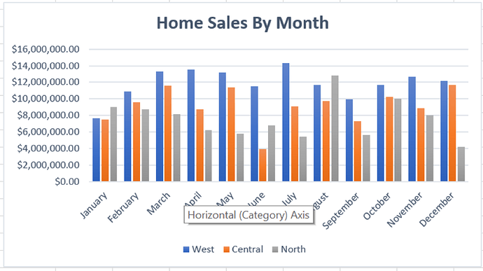
Construct a column chart based on your completed data table. It should have the following:

Three data series: one for the sales in each region (West, Central, and North)
“Month” on the horizontal/category axis
A legend below the chart to identify each series
A title above the chart reading “Home Sales By Month”
Additional formatting/built-in styles of your choice

Your chart should look something like this:

Exercise 4

Create a copy of the “Exercise 3” worksheet, and name it “Exercise 4”.
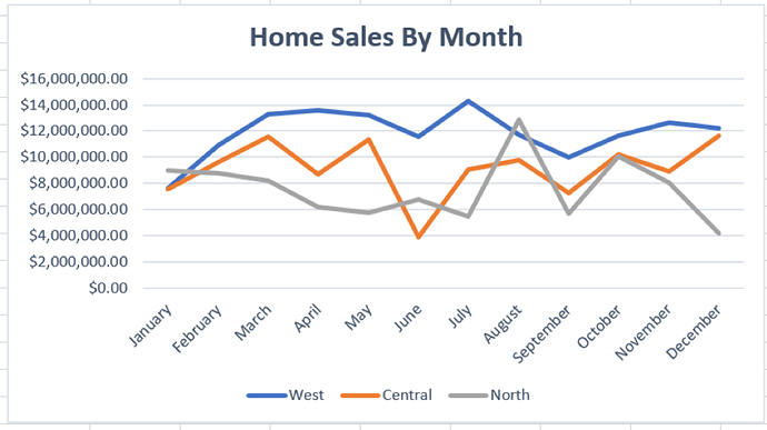
Change the column chart on the new worksheet to be a line chart instead

Your chart should look something like this:

Exercise 5

On the “Exercise 5” worksheet , use the AVERAGEIFS function to populate the “Average Square Footage” column with the average square footage (from the “SquareFootage” column on the “Home Sale Data” worksheet) for each month.
Then, use the SUMIFS function to populate the “Total Sales” column with the total sales (from the “SalePrice” column on the “Home Sale Data” worksheet) for each month.
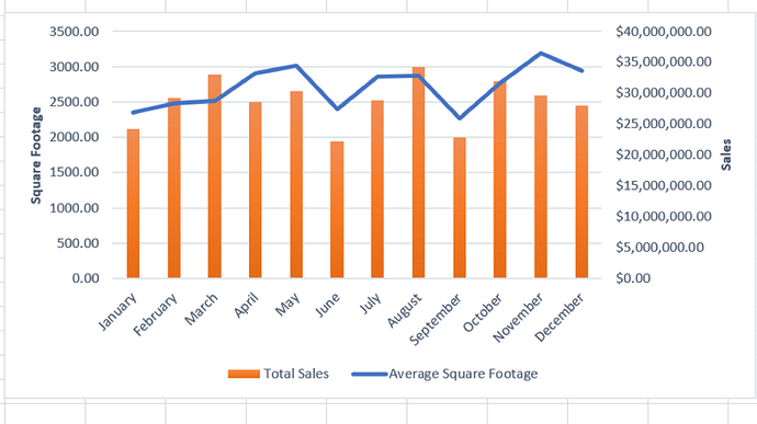
Construct a combination column/line chart based on your completed data table. It should have the following:

Two data series: one for average square footage, and one for total sales
“Month” on the horizontal/category axis
Average square footage should be plotted against the primary axis, as a line chart.
Total sales should be plotted against the secondary axis, as a column chart.
There should be a legend below the chart to identify each series.
Both the primary and secondary vertical axes should have titles.
Feel free to include additional formatting/built-in styles of your choice.

The chart should look something like this:

Exercise: Working With Structure Data in Excel

That’s right, we’re importing and using external data now, woooooooo! You got this!

Exercise: Working With Structured Data

Download and open the “Working With Structured Data - Starter.xlsx” file (it’s at the bottom of this page, like usual).

Exercise 1

On the “Exercise 1” worksheet , use Excel’s Text to Columns feature to split the data in column A into distinct columns. HINT: you’ll need to use a different delimiter than a comma!

Exercise 2

Download and open the “External Data Files.zip” file at the bottom of this page.
Within that zip file, open the “External Data 1.csv” file .
Save the file to some location on your computer (the specific folder doesn’t matter, just remember it for the next step!).
Using Excel’s menu for working with external data, import the contents of the “External Data.csv” file into the “Working With Structured Data - Starter.xlsx” file.
Name the resulting Excel Table “home_sale_data”.

Exercise 3

Open again the “External Data Files.zip” file and go to the External Data 2.csv" file within
Save the file over the .csv file you saved in Exercise 2 - in other words, the name of the saved file should be “External Data.csv”.
Take note of how many rows of data are currently in the “home_sale_data” table.
Refresh the data source for the the “home_sale_data” table. Does the number of rows in the table change?

Exercise 4

In the “home_sale_data” table, insert a blank column to the right of the “SalePrice” column. Give the column the name “AgentCommission”.
Populate this new column with a formula that returns 5% of the number in the “SalePrice” column (i.e., multiplies it by 0.05). Make sure your formula is “table style”, referencing table columns instead of cell references.

Exercise 5

Navigate to the “Regions” worksheet ; convert the range of values in columns A and B to an Excel table . Name the table “regions”.
Back in the “home_sale_data” table, insert a blank column to the right of the “City” column. Give the column the name “Region”.
Keying off the values in the “City” column, use a VLOOKUP function to pull the region values from your newly-created lookup table into the blank “Region” column.
Scan the values in the “Region” column for errors - you will probably notice some for records where the city is “Lexington”.
Go back to the “Regions” worksheet , and add the following values at the bottom of the table:
“Lexington”, in the “City” column
“Central”, in the “Region” column
Reassess the “Region” column in the “home_sale_data” table - are the errors still there?

Exercise: Pivot Tables

“It’s not who I am underneath, but what I do that defines me.” - Batman.

That’s right, Batman said this quote. And he was actually talking specifically about doing Excel Pivot Tables when he said it. He’s a big Excel guy in case you didn’t know. Be like Batman.

Exercises: Pivot Tables

Download and open the “Pivot Tables - Starter.xlsx” file at the bottom of this page .

Exercise 1

Select the entire “home_sale_data” Table on the “Data” worksheet .
Insert a Pivot Table based on this Table into a new worksheet .
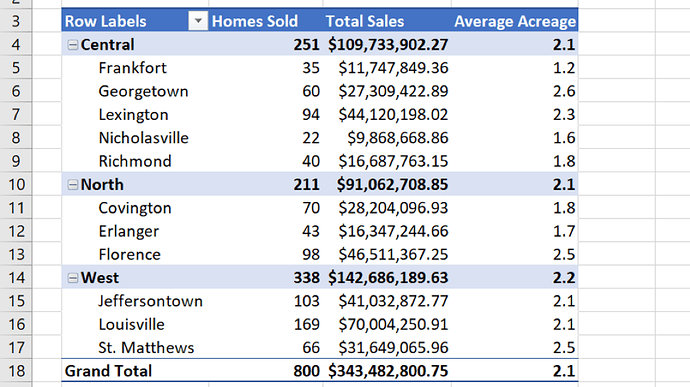
Drag in fields from the source data such that the Pivot Table is structured like the example below:

Use any field you like as the basis for the the “Homes Sold” field, but make sure it is summarized as a count .
“SalePrice” should be summarized by sum .
“Acreage” should be summarized by average .

Exercise 2

Update the “Homes Sold” field to summarize the count as a percentage of the parent row total.

Exercise 3

Add a new metric to the Pivot Table called “% of Sales > 500K” that displays the percent of home sales that were over $500,000.

HINTS:

Try adding a 1/0 field to the Table the Pivot Table is sourced from, which evaluates whether a sale price was greater than $500,000.
Then, this field can be summarized in the Pivot Table as an average, with the result being formatted as a percent.
Don’t forget to refresh your Pivot Table so you can see the new field!

Exercise 4

Copy your Pivot Table, and paste the copy directly to the right of it.
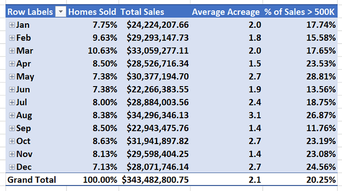
Remove “City” and “Region” from the copied Pivot Table, and replace with “SaleDate”
Make sure “SaleDate” is grouped by day AND month.
Make sure the “Months” group is collapsed so that the Pivot Table looks like this:

Exercise 5

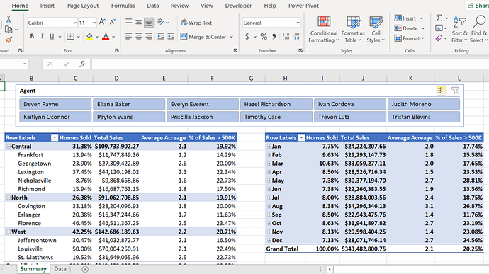
Insert enough blank rows above both Pivot Tables to make room for a Slicer.
Add a Slicer above the Pivot Table for the “Agent” field.
Orient the Slicer values into multiple columns (I would suggest six) to make better use of space on the worksheet.
Make sure that the Slicer is connected to both Pivot Tables.
Try applying some single and multi-valued filters to the Slicer.

Your solution should look something like this:

Exercise: Macros and VBA

Gimme a V! Gimme a B! Gimme an A! What’s that spell? VBA!

Exercise: VBA Macros

Part 1

Even if you skipped the “Excel 101” section of the course , take a moment to review the exercises at the end of that section. We’re going to be automating most of these steps with a VBA macro!

After acquainting yourself with those steps, download and open the “Macros - Starter.xlsx” file that’s at the bottom of this page.

Part 2

Within the “Macros - Starter.xlsx” file , record a macro in the to capture the following actions:

Delete the “ProductID” column in the data.
Unmerge the two cells composing the “CustomerName” column header, and then add “Customer First Name” and “Customer Last Name” headers for the two columns.
Cut the “Customer First Name” and “Customer Last Name” columns, and insert them to the left of the “ReviewStars” column.
Edit the remaining column headers to have spaces between the words in the names (i.e, “ProductName” becomes “Product Name”).
Insert a new column, to the left of the other columns, and give it a column header of “Review Number”.
Using Excel’s autofill feature, populate this column with a series of numbers from one to the number of reviews in the dataset.
Re-format the “Purchase Date” and “Review Date” columns to the MM/DD/YYYY date format.
Re-format the “Review Stars” column to display zero digits after the decimal place.
Using Excel’s find and replace feature, replace all instances of the word “ukelele” on the worksheet with “ukulele”.
Change the font of all the cells in the range to “Segoe UI”, size 10.
Give the column headers a dark background fill color from one of Excel’s built-in “theme” colors - your choice!
Change the font color of the column headers to white.
Bold the column headers.
Auto-fit the widths of the columns to adjust to the width of the data they contain.
Freeze the top row of the data (the column headers) so that it remains visible no matter how far you scroll down through the data.
Finally, stop recording the macro.

Part 3

Edit the macro code as follows:

Fix any missteps you made while recording (if any), that Excel captured in the VBA code.
Remove any extraneous lines of VBA code the were generated by actions you don’t need to capture.
Have the macro name the “Review Number” column “Review ID” instead.
Add a line of code of code at the beginning of the macro that suppresses alerts/warnings/dialog boxes for the duration of the macro.
Add a line of code at the end of the macro that causes a message box to appear after the macro completes, which says: “Congratulations, your macro ran successfully!”.
Save the file as “Customer Reviews Template.xlsm” (note the macro-enabled file format) . This is now your template file.

Part 4

Delete all the columns containing data on the worksheet.
Unfreeze panes in the worksheet.
Add a button to the worksheet, and assign it to your “ProcessData” macro.
Give the button a caption of “Execute Process”.
Make sure the button is positioned far enough to the right to allow room for us to copy and paste in new data.
Save the template file (don’t want to lose your changes!).

Part 5

Time to put your template file to the test!

Re-open the “Macros - Starter.xlsx” file in the resources section below.
Copy and paste the data from the “Macros - Starter.xlsx” file into cell A1 of our template file .
Click your “Execute Process” button, and hope for the best!
If anything goes awry, edit the macro code and see if you can diagnose the issue.